How AI Understands Images: Vision Transformers Explained

The first time I tried to explain to a colleague how GPT-4o "sees" an image, I said something like "it converts the image into tokens, similar to how it tokenises text." He thought I was being reductive. Then I showed him the actual ViT paper, and we both stared at the architecture diagram for a while. It really is that direct. An image gets cut into a grid of fixed-size patches. Each patch becomes a vector. Those vectors go into a transformer. The transformer does attention. That is the whole story, and it is remarkable that something so conceptually simple outperforms 20 years of convolutional network research on most tasks.

This post is for engineers who already know how transformers work on text and want to understand how the same architecture handles images. I will go from the original ViT paper's idea through CLIP and vision-language models to the practical details that affect your code today.

Why convolutions stopped being enough

Convolutional neural networks (CNNs) dominated computer vision from roughly 2012 (AlexNet) to 2020. The core idea: slide a small filter over an image, multiply each pixel by the filter weights, sum the result. Stack many such layers, and the network learns to detect edges, then shapes, then objects. CNNs have useful inductive biases baked in — translation equivariance (the same object anywhere in the image activates the same filter) and local connectivity (each filter looks at a small neighbourhood, not the whole image).

Those inductive biases are also CNN's limitations. They struggle to model long-range dependencies. To detect that the object in the top-left corner relates to the object in the bottom-right corner, a CNN has to stack enough layers that the receptive field eventually spans the full image. That is expensive in depth and compute.

Transformers have no such constraint. Self-attention computes relationships between every position and every other position in a single operation. If you can get an image into a form that a transformer can process, it can model relationships across the full spatial extent of the image in the very first layer.

The question was how to get there.

The ViT insight: treat image patches as tokens

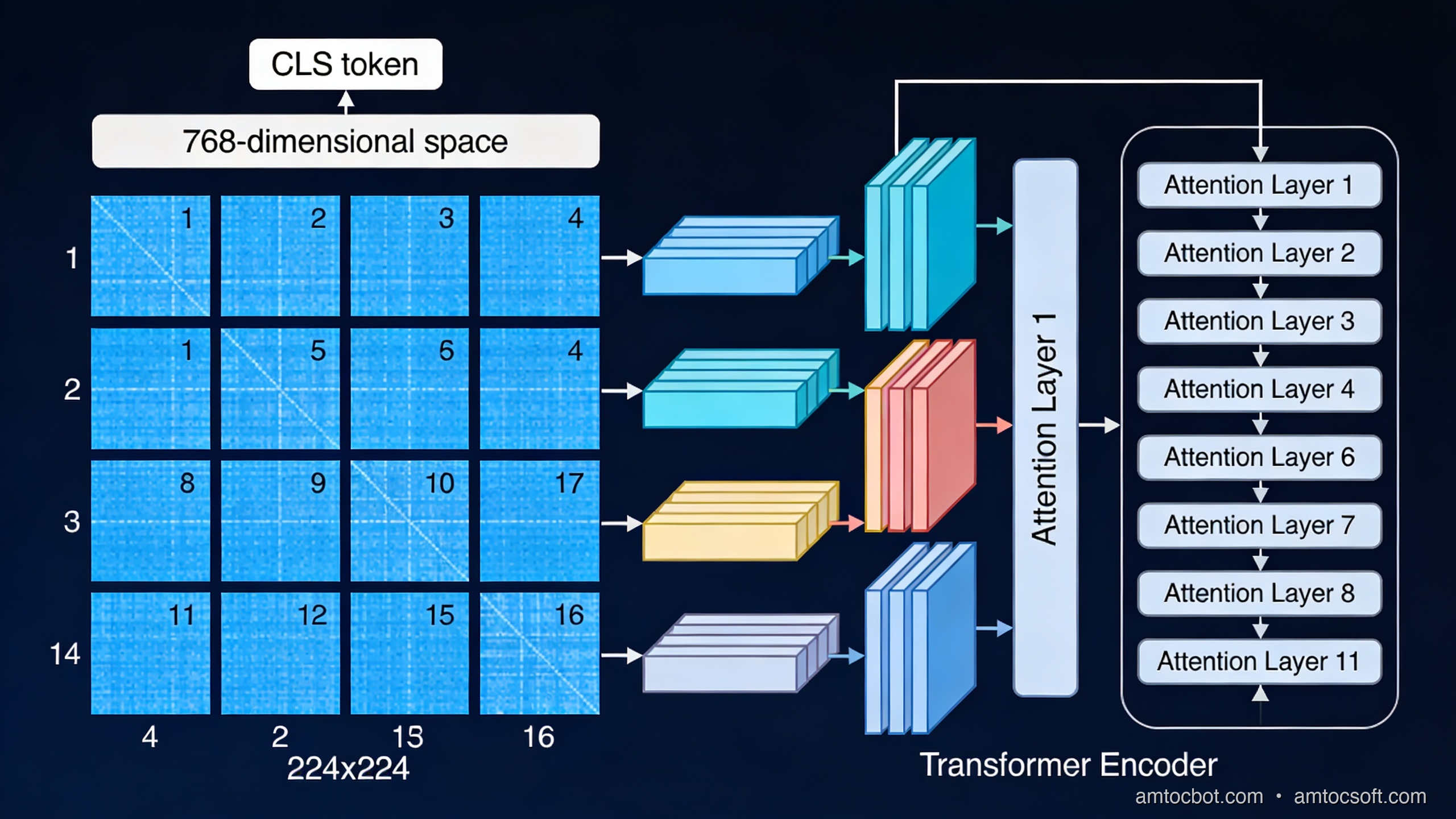
The Vision Transformer paper (Dosovitskiy et al., "An Image is Worth 16x16 Words", 2020) had an elegant answer. If a language transformer processes sequences of token vectors, you just need to convert an image into a sequence of vectors. Here's how:

1. Divide the input image into a regular grid of non-overlapping patches. The original ViT uses 16×16 pixel patches, giving 196 patches for a 224×224 image.
2. Flatten each patch into a 1D vector. A 16×16 RGB patch flattens to 16 × 16 × 3 = 768 values.
3. Project each flat vector through a learned linear layer to produce a patch embedding of fixed dimension (768 in ViT-Base).
4. Prepend a learnable [CLS] token (borrowed from BERT), whose output representation the model uses for classification.
5. Add positional embeddings to each patch vector so the model knows where in the image each patch came from.
6. Feed the resulting sequence of N+1 vectors into a standard transformer encoder.

The transformer's self-attention operates across all N+1 positions simultaneously. A patch near the top-left can directly attend to a patch near the bottom-right in the first layer. There is no CNN's stacking requirement.

import torch
import torch.nn as nn

class PatchEmbedding(nn.Module):
    """
    Converts an image tensor into a sequence of patch embeddings.

    input:  (B, C, H, W)  — batch of images
    output: (B, N, D)     — batch of N patch embeddings of dimension D
    """
    def __init__(
        self,
        image_size: int = 224,
        patch_size: int = 16,
        in_channels: int = 3,
        embed_dim: int = 768,
    ):
        super().__init__()
        self.num_patches = (image_size // patch_size) ** 2
        # A single Conv2d with kernel_size=patch_size and stride=patch_size
        # is equivalent to flattening + projecting each patch.
        self.projection = nn.Conv2d(
            in_channels,
            embed_dim,
            kernel_size=patch_size,
            stride=patch_size,
        )

    def forward(self, x: torch.Tensor) -> torch.Tensor:
        # x: (B, C, H, W)
        x = self.projection(x)  # (B, embed_dim, H/patch, W/patch)
        x = x.flatten(2)        # (B, embed_dim, N)
        x = x.transpose(1, 2)  # (B, N, embed_dim)
        return x

# Example
embed = PatchEmbedding()
img = torch.randn(1, 3, 224, 224)
patches = embed(img)
print(patches.shape)  # torch.Size([1, 196, 768])

The Conv2d trick is elegant: using a convolution with kernel_size=patch_size and stride=patch_size is computationally equivalent to flattening each patch and multiplying by a weight matrix, but it reuses the GPU's optimised convolution paths.

Self-attention over image patches

Once you have your sequence of 196 patch embeddings (plus the CLS token = 197 total), the transformer encoder runs exactly as it does for text. Each attention head computes:

Attention(Q, K, V) = softmax(QK^T / √d_k) V

Where Q, K, V are linear projections of the input. For a multi-head attention layer with 12 heads and 768 embedding dimension, each head operates on 64-dimensional projections.

What does attention over patches actually compute? Empirically, earlier transformer layers tend to show attention patterns that focus on nearby patches — similar to local CNN receptive fields, but learned rather than hardcoded. Deeper layers show long-range attention patterns that span the full image: the attention map of a patch showing a person's face may light up another patch showing that person's hands if they're relevant to the classification task.

This is measurable. Caron et al. (DINO, 2021) visualised the attention maps of a self-supervised ViT and showed that the model learns to segment objects from backgrounds without any segmentation training signal — purely from classification-style self-supervision. The multi-head attention mechanism naturally specialises different heads for different semantic groupings.

flowchart TD
    A[Input Image 224×224] --> B[Divide into 196 patches of 16×16]
    B --> C[Flatten each patch to 768-dim vector]
    C --> D[Add learned positional embedding]
    D --> E[Prepend CLS token]
    E --> F[Transformer Encoder × 12 layers]
    F --> G[Multi-Head Self-Attention<br/>12 heads, 64 dim each]
    G --> H[MLP Block<br/>768 → 3072 → 768]
    H --> I{Need global feature?}
    I -->|Yes - classification| J[CLS token output → Linear → Logits]
    I -->|No - dense features| K[All patch tokens → feature map]

ViT vs CNN: when does each win?

This was the nuanced result from the original ViT paper that most coverage missed. ViT does not automatically beat CNNs. The competitive behaviour depends heavily on dataset size:

Training data	ViT-Large vs ResNet-152
ImageNet only (1.2M images)	ResNet wins: ViT underfits
ImageNet-21k (14M images)	Roughly equal
JFT-300M (300M images)	ViT wins clearly
JFT-300M + fine-tune ImageNet	ViT-Large: 88.55% top-1

The reason: CNNs' inductive biases (local connectivity, translation equivariance) are actually a form of built-in knowledge about images. They help when training data is limited. ViT's fully general attention has to learn those biases from data — which requires more data, but can ultimately learn more flexible representations.

For most production applications, the practical answer since 2022 is: use a pre-trained ViT that has already seen hundreds of millions of images. Fine-tuning on your downstream task inherits the general visual representations. The original data-scale limitation is not your problem at inference time.

CLIP: connecting vision and language

CLIP (Contrastive Language-Image Pretraining, OpenAI 2021) is the component that made vision transformers practical for open-ended tasks. The key insight: train a vision encoder and a text encoder jointly, using contrastive loss to align their representations.

Training procedure:
- For each (image, text) pair in the training batch, encode both with their respective encoders.
- Compute cosine similarity between all N×N pairs in the batch.
- Train so that the N matching (image, text) pairs have high similarity; all N²-N non-matching pairs have low similarity.

OpenAI trained CLIP on 400 million (image, text) pairs scraped from the web. The result: the vision encoder learns to produce representations that capture semantic content, not just visual features. Two photos of the same concept produce similar embeddings, even if they look visually very different.

flowchart LR
    A["Photo of a cat"] --> B[ViT Vision Encoder]
    B --> C[Image Embedding\n512-dim normalised]
    D["Text: 'a photo of a cat'"] --> E[Text Transformer]
    E --> F[Text Embedding\n512-dim normalised]
    C <-->|"cosine similarity\nmaximised for matching pairs\nminimised for non-matching"| F
    G["Text: 'a dog running'"] --> H[Text Transformer]
    H --> I[Text Embedding]
    C <-->|"low similarity"| I

Zero-shot classification with CLIP:

from PIL import Image
import requests
import torch
from transformers import CLIPProcessor, CLIPModel

model = CLIPModel.from_pretrained("openai/clip-vit-base-patch32")
processor = CLIPProcessor.from_pretrained("openai/clip-vit-base-patch32")

# Load an image
url = "http://images.cocodataset.org/val2017/000000039769.jpg"
image = Image.open(requests.get(url, stream=True).raw)

# Define candidate labels as free-form text
labels = [
    "a photo of a cat",
    "a photo of a dog",
    "a photo of a bird",
    "a photo of a car",
]

inputs = processor(
    text=labels,
    images=image,
    return_tensors="pt",
    padding=True,
)

with torch.no_grad():
    outputs = model(**inputs)

# Image-text similarity scores, softmaxed to probabilities
logits = outputs.logits_per_image  # shape: (1, num_labels)
probs = logits.softmax(dim=-1).squeeze()

for label, prob in zip(labels, probs):
    print(f"{label}: {prob:.3f}")

# Output (approximate):
# a photo of a cat: 0.914
# a photo of a dog: 0.031
# a photo of a bird: 0.041
# a photo of a car: 0.014

No fine-tuning. No labelled training data. You can add new classes at inference time just by writing new text descriptions. This is the practical superpower of CLIP-style models: zero-shot generalisation to new visual concepts via natural language.

How this connects to GPT-4o and Claude

Modern multimodal LLMs use CLIP or CLIP-like vision encoders as the "eyes" that feed into a large language model. The architecture varies by system, but the broad pattern:

flowchart LR
    A[Input Image] --> B[CLIP Vision Encoder\nor ViT variant]
    B --> C[Visual Features\nN patch embeddings]
    C --> D[Projection Layer\naligns vision dim → LLM dim]
    E[Text Tokens] --> F[Text Tokeniser]
    D --> G[Interleaved Token Sequence]
    F --> G
    G --> H[Large Language Model\nGPT-4o / Claude / Gemini]
    H --> I[Output Text]

GPT-4o's vision encoder takes the image, generates patch-level features, and those features get projected into the same embedding dimension as the text tokens. The LLM then processes the combined sequence via its standard transformer attention. From the language model's perspective, image regions are just different tokens — which is why it can answer questions like "what's written in the top-right corner?" by attending to the relevant patch tokens.

One detail that matters for performance: the projection layer between the vision encoder and the language model is critical. LLaVA (Liu et al., 2023) showed that a simple linear projection works well at scale; other approaches like Flamingo (DeepMind) use cross-attention layers. The tradeoff is efficiency vs representational power. For GPT-4o-scale deployments, a linear projection keeps inference fast while the sheer scale of pretraining compensates for the architectural simplicity.

The gotcha that cost me two days: positional embedding failure on out-of-distribution image sizes

The original ViT trains with fixed-size images (224×224 = 196 patches). The positional embeddings are fixed at 197 positions (196 patches + CLS). What happens when you feed a 512×512 image at inference time?

The ViT paper handles this with positional embedding interpolation: the 14×14 grid of trained position embeddings gets bicubically interpolated to whatever grid size you need. This is built into most implementations via interpolate_pos_encoding.

In production, I discovered this the hard way. We had a ViT-based image classifier that performed well in testing on 224×224 crops. When we switched to feeding full-resolution 1024×768 images (resized to 1024×768, not cropped to 224×224), accuracy dropped from 91% to 73%. The model was generating a 64×48 = 3072 patch grid, and while the positional embeddings were technically interpolated, the distribution shift from 14×14 training grids to 64×48 inference grids was severe enough to degrade the early-layer features significantly.

The fix: fine-tune with native resolution augmentation, or use a model like ViT-L/14@336px that was trained at higher resolution, or use DINOv2 which handles resolution changes more robustly due to its self-supervised training approach.

# Check if your ViT supports flexible resolution
from transformers import ViTModel

model = ViTModel.from_pretrained("google/vit-base-patch16-224")

# This will raise or silently produce wrong results 
# if the model was not trained/fine-tuned for this size:
import torch
dummy_input = torch.randn(1, 3, 512, 512)

# Safe approach: always check patch_size divisibility
assert 512 % model.config.patch_size == 0, (
    f"Image size 512 not divisible by patch_size {model.config.patch_size}"
)

# And verify the model was trained with interpolation support
print(model.config.interpolate_pos_encoding)  # Should be True

Production considerations

Inference speed: ViT attention is O(N²) in sequence length. A 224×224 image with patch_size=16 gives N=196, which is fast. A 1024×1024 image with patch_size=16 gives N=4096 — 441× more attention operations. Use patch_size=32 or hierarchical vision models (Swin Transformer) for high-resolution inputs.

Swin Transformer: Microsoft Research's answer to the resolution problem. Instead of global self-attention over all patches, Swin uses local window attention (each patch attends only to its 7×7 window neighbourhood) plus a shifting window scheme that allows cross-window information to flow. This reduces attention complexity from O(N²) to O(N) with respect to image size, at the cost of less global attention in early layers.

DINOv2 (Meta AI, 2023): Currently the best off-the-shelf vision encoder for downstream fine-tuning tasks. Trained with self-supervised learning on curated data (LVD-142M), it produces dense visual features that transfer extremely well to segmentation, depth estimation, and classification without any task-specific pretraining. DINOv2 ViT-L achieves 86.3% top-1 on ImageNet with linear probing — no fine-tuning of the vision encoder at all.

Memory at training time: Full ViT attention on large images is expensive in GPU memory. Standard approaches: gradient checkpointing (trade compute for memory), mixed precision training (bfloat16 on H100/A100), and FlashAttention (reduces attention memory from O(N²) to O(N) via IO-aware tiling).

When to use what

Use case	Recommended approach
Image classification, well-resourced	Fine-tune DINOv2 or ViT-L/16 pre-trained
High-resolution input (>512px)	Swin-L or ViT with patch_size=32
Zero-shot visual understanding	CLIP ViT-L/14 or SigLIP
Dense prediction (segmentation, depth)	DINOv2 + task head
Production multimodal LLM	Use cloud API (GPT-4o, Claude 3.5) rather than running ViT yourself
Edge / mobile inference	EfficientNet or MobileViT — not standard ViT

Conclusion

Vision Transformers work because the transformer architecture makes no assumptions about the modality of its input — only that the input is a sequence of fixed-dimension vectors. Images become sequences via patch tokenization. The self-attention mechanism then has the ability to model arbitrary long-range dependencies across the image from the very first layer, which CNN stacking cannot match.

CLIP extended this by training vision encoders jointly with language encoders, creating a shared semantic space where image patches and text tokens occupy the same representational territory. That shared space is what modern multimodal LLMs exploit: the ViT produces patch tokens that slot into the same sequence as text tokens, letting the language model reason across both.

The practical path for most engineering teams is clear: use pre-trained models (DINOv2, CLIP, or hosted APIs like GPT-4o) rather than training vision transformers from scratch. The representational quality from large-scale pretraining is hard to replicate at project timescales. Understand the architecture so you can debug it when production breaks — and it will break at image resolutions you didn't test.

Sources

1. Dosovitskiy et al. (2020), "An Image is Worth 16x16 Words: Transformers for Image Recognition at Scale" — https://arxiv.org/abs/2010.11929
2. Radford et al. (2021), "Learning Transferable Visual Models From Natural Language Supervision (CLIP)" — https://arxiv.org/abs/2103.00020
3. Oquab et al. (2023), "DINOv2: Learning Robust Visual Features without Supervision" — https://arxiv.org/abs/2304.07193

About the Author

Toc Am

Founder of AmtocSoft. Writing practical deep-dives on AI engineering, cloud architecture, and developer tooling. Previously built backend systems at scale. Reviews every post published under this byline.

LinkedIn X / Twitter

Published: 2026-04-29 · Written with AI assistance, reviewed by Toc Am.

☕ Buy Me a Coffee · 🔔 YouTube · 💼 LinkedIn · 🐦 X/Twitter