Showing posts with label optimization. Show all posts

Wednesday, April 15, 2026

Database Query Optimization: EXPLAIN ANALYZE, Indexes, and the Queries That Kill Production

Hero: EXPLAIN ANALYZE output with cost breakdown and slow query highlighted

A database query that runs in 3ms with 1,000 rows will often take 4,000ms with 1,000,000 rows. The query didn't change. The data changed. Most production database incidents aren't caused by code bugs — they're caused by queries that worked fine in staging (with 5,000 rows) and collapsed in production (with 50,000,000 rows).

This guide covers the tools and patterns for diagnosing and fixing slow queries in PostgreSQL and MySQL: reading query plans, choosing the right indexes, eliminating N+1 queries, and avoiding the schema patterns that guarantee future pain.

The Problem: Queries That Look Fine But Aren't

Consider this query:

SELECT u.name, u.email, COUNT(o.id) as order_count
FROM users u
LEFT JOIN orders o ON o.user_id = u.id
WHERE u.created_at > '2025-01-01'
GROUP BY u.id, u.name, u.email
ORDER BY order_count DESC
LIMIT 20;

In development with 500 users and 2,000 orders: 4ms. In production with 2M users and 80M orders: 45 seconds. A sequential scan of 80M rows, a hash join, and a sort of 2M groups — all because there's no index on orders.user_id and users.created_at.

The tools to find and fix this exist in every database. Most developers don't know how to read them.

How It Works: Reading EXPLAIN ANALYZE

EXPLAIN ANALYZE is the most important debugging tool for slow queries. It shows the query plan the database chose and the actual execution statistics.

EXPLAIN (ANALYZE, BUFFERS, FORMAT TEXT)
SELECT u.name, u.email, COUNT(o.id) as order_count
FROM users u
LEFT JOIN orders o ON o.user_id = u.id
WHERE u.created_at > '2025-01-01'
GROUP BY u.id, u.name, u.email
ORDER BY order_count DESC
LIMIT 20;

Sample output (annotated):

Limit  (cost=248542.33..248542.38 rows=20 width=48) (actual time=44812.221..44812.226 rows=20 loops=1)
  ->  Sort  (cost=248542.33..253447.89 rows=1962224 width=48) (actual time=44812.219..44812.221 rows=20 loops=1)
        Sort Key: (count(o.id)) DESC
        Sort Method: top-N heapsort  Memory: 26kB
        ->  HashAggregate  (cost=185899.07..205521.31 rows=1962224 width=48) (actual time=38211.442..43187.553 rows=1962224 loops=1)
              Group Key: u.id
              Batches: 5  Memory Usage: 4145kB  Disk Usage: 36608kB  ← SPILLING TO DISK
              ->  Hash Left Join  (cost=44729.61..163355.95 rows=4508624 width=24) (actual time=1203.442..28847.221 rows=80124532 loops=1)
                    Hash Cond: (o.user_id = u.id)
                    ->  Seq Scan on orders o  (cost=0.00..82441.32 rows=4508624 width=8) (actual time=0.021..8442.112 rows=80124532 loops=1)
                                                                                                                          ↑ SEQUENTIAL SCAN — 80M rows
                    ->  Hash  (cost=29972.87..29972.87 rows=1182939 width=24) (actual time=1190.221..1190.221 rows=1962224 loops=1)
                          Buckets: 2097152  Batches: 2  Memory Usage: 50421kB
                          ->  Seq Scan on users u  (cost=0.00..29972.87 rows=1182939 width=24) (actual time=0.012..892.442 rows=1962224 loops=1)
                                Filter: (created_at > '2025-01-01 00:00:00'::timestamp)
                                Rows Removed by Filter: 37776                     ← Only removes 37K rows from 2M scan
Planning Time: 2.442 ms
Execution Time: 44814.221 ms  ← 44 seconds

The key numbers to read:

What to look for Where it is What it means
Seq Scan on large table Node type Missing index — table scanned row by row
High actual time vs cost Each node Planner estimate was wrong
Disk Usage in aggregation HashAggregate Query spilling to disk — work_mem too low
Rows Removed by Filter Seq Scan Filter applied after reading all rows
loops=N where N > 1 Nested Loop Inner relation scanned N times
flowchart TD A[EXPLAIN ANALYZE output] --> B{Seq Scan?} B -- Yes on large table --> C[Add index on scan columns] B -- No --> D{Nested Loop with loops > 100?} D -- Yes --> E[N+1 query or missing join index] D -- No --> F{Disk Usage in aggregation?} F -- Yes --> G[Increase work_mem or optimize grouping] F -- No --> H{High actual vs estimated rows?} H -- Yes --> I[Run ANALYZE to update statistics] H -- No --> J[Query is probably fine] style C fill:#ef4444,color:#fff style E fill:#ef4444,color:#fff style G fill:#f59e0b,color:#fff style I fill:#f59e0b,color:#fff style J fill:#22c55e,color:#fff

Implementation: Fixing the Common Culprits

Fix 1: Add the Right Indexes

The query above needs two indexes:

-- Index for the WHERE clause on users
CREATE INDEX idx_users_created_at ON users(created_at);

-- Index for the JOIN condition on orders  
CREATE INDEX idx_orders_user_id ON orders(user_id);

After adding these, EXPLAIN ANALYZE shows:

Execution Time: 312 ms   ← Down from 44,814ms

Choosing index types:

-- B-tree (default): range queries, equality, ORDER BY
CREATE INDEX idx_orders_created_at ON orders(created_at);  -- WHERE created_at > '...'

-- Hash: equality only (faster for = than B-tree, no range support)
-- PostgreSQL 10+ only, rarely needed
CREATE INDEX idx_orders_status_hash ON orders USING HASH (status);

-- Partial index: index only rows that match a condition
-- Smaller index, faster for filtered queries
CREATE INDEX idx_orders_pending ON orders(user_id) 
    WHERE status = 'pending';  -- Only indexes pending orders

-- Composite index: column order matters
-- This index helps: WHERE user_id = ? AND created_at > ?
-- Also helps: WHERE user_id = ?  (leading column)
-- Does NOT help: WHERE created_at > ?  (non-leading column)
CREATE INDEX idx_orders_user_created ON orders(user_id, created_at);

-- Covering index: include non-indexed columns to avoid table heap access
-- Query only touches the index, never the table
CREATE INDEX idx_orders_covering ON orders(user_id, created_at) 
    INCLUDE (status, total_amount);

The most common mistake: Creating an index on a column used in a WHERE clause when the column has low cardinality. An index on status where status is one of three values ('pending', 'active', 'closed') helps nothing — the planner will still do a sequential scan because 33% of rows match, and a seq scan is faster than reading 33M index entries.

-- WRONG: low cardinality, index will be ignored
CREATE INDEX idx_users_is_active ON users(is_active);  -- Only 2 values

-- RIGHT: high cardinality, or restrict with partial index
CREATE INDEX idx_users_active ON users(id) WHERE is_active = true;
-- Now a small index covering only active users

Fix 2: The N+1 Query Destroyer

N+1 is the single most common database performance problem in ORMs. The pattern:

# ORM code that looks innocent
users = User.objects.filter(created_at__gt='2025-01-01')

for user in users:
    # THIS IS N+1 — one query per user
    print(user.orders.count())

What happens: 1 query to get N users, then N queries to get each user's order count. With 10,000 users: 10,001 database round trips. At 2ms per round trip: 20 seconds.

-- What the ORM is running (10,001 queries):
SELECT * FROM users WHERE created_at > '2025-01-01';
SELECT COUNT(*) FROM orders WHERE user_id = 1;
SELECT COUNT(*) FROM orders WHERE user_id = 2;
-- ... × 9,999 more

The fix: annotate or JOIN to get everything in one query:

# Django: annotate with COUNT in a single query
from django.db.models import Count

users = (
    User.objects
    .filter(created_at__gt='2025-01-01')
    .annotate(order_count=Count('orders'))
    .order_by('-order_count')[:20]
)
# 1 query total: the JOIN + COUNT SQL from earlier
# SQLAlchemy: same idea
from sqlalchemy import func

result = (
    session.query(User, func.count(Order.id).label('order_count'))
    .outerjoin(Order, Order.user_id == User.id)
    .filter(User.created_at > '2025-01-01')
    .group_by(User.id)
    .order_by(desc('order_count'))
    .limit(20)
    .all()
)

Detecting N+1 in production:

# Django Debug Toolbar shows query count per request
# For production monitoring, track queries-per-request in your APM

# Or log slow query patterns manually:
import django.db.backends.utils as db_utils
import logging

original = db_utils.CursorWrapper.execute

def patched_execute(self, sql, params=None):
    logging.debug(f"QUERY: {sql[:200]}")
    return original(self, sql, params)

db_utils.CursorWrapper.execute = patched_execute

Fix 3: JSONB Performance (PostgreSQL)

Storing semi-structured data in JSONB columns is convenient but has performance traps:

-- SLOW: no index on JSONB field, full table scan
SELECT * FROM events WHERE metadata->>'user_id' = '12345';

-- FIX 1: GIN index on entire JSONB column (handles any key lookup)
CREATE INDEX idx_events_metadata_gin ON events USING GIN (metadata);

-- FIX 2: Expression index on specific key (smaller, faster for single key)
CREATE INDEX idx_events_user_id ON events((metadata->>'user_id'));

-- FIX 3: If you always query the same keys, use a generated column
ALTER TABLE events 
ADD COLUMN user_id_extracted TEXT 
    GENERATED ALWAYS AS (metadata->>'user_id') STORED;
CREATE INDEX idx_events_user_id_col ON events(user_id_extracted);
-- Now it's just a regular column with a regular index

Fix 4: The Pagination Trap

OFFSET-based pagination is fine with small datasets. With large ones, it's a silent killer:

-- SLOW: scans and discards 999,980 rows to return rows 999,981-1,000,000
SELECT * FROM events ORDER BY created_at DESC LIMIT 20 OFFSET 999980;

-- FIX: cursor-based pagination using the last seen ID
-- First page:
SELECT * FROM events ORDER BY created_at DESC, id DESC LIMIT 20;

-- Subsequent pages (pass last_created_at and last_id from previous response):
SELECT * FROM events 
WHERE (created_at, id) < ('2025-06-15 10:23:44', 98765)
ORDER BY created_at DESC, id DESC 
LIMIT 20;

The cursor approach scans exactly 20 rows regardless of which page you're on. The OFFSET approach scans N+20 rows every time.

Query Patterns to Avoid

flowchart LR A[Dangerous Patterns] A --> B["SELECT * (fetches all columns)"] A --> C["WHERE LOWER(email) = ... (function prevents index use)"] A --> D["WHERE id::text = '123' (cast prevents index use)"] A --> E["LIKE '%search%' (leading wildcard = seq scan)"] A --> F["OR conditions on different columns (index skipped)"] B --> B2["SELECT only needed columns"] C --> C2["Use citext column type or expression index"] D --> D2["Match column type in WHERE clause"] E --> E2["Full-text search (tsvector/tsquery)"] F --> F2["Separate queries with UNION ALL"] style A fill:#ef4444,color:#fff
-- FUNCTION IN WHERE: prevents index use
-- SLOW:
SELECT * FROM users WHERE LOWER(email) = 'user@example.com';

-- FIX: use citext extension for case-insensitive storage
CREATE EXTENSION IF NOT EXISTS citext;
ALTER TABLE users ALTER COLUMN email TYPE citext;
-- Now: WHERE email = 'USER@EXAMPLE.COM' uses the index

-- OR: use an expression index
CREATE INDEX idx_users_email_lower ON users(LOWER(email));
SELECT * FROM users WHERE LOWER(email) = 'user@example.com';  -- Now uses index


-- LEADING WILDCARD: full table scan
-- SLOW:
SELECT * FROM products WHERE name LIKE '%widget%';

-- FIX: full-text search with GIN index
ALTER TABLE products ADD COLUMN search_vec tsvector
    GENERATED ALWAYS AS (to_tsvector('english', name || ' ' || description)) STORED;
CREATE INDEX idx_products_search ON products USING GIN(search_vec);
SELECT * FROM products WHERE search_vec @@ plainto_tsquery('english', 'widget');

VACUUM, Bloat, and Table Maintenance

PostgreSQL doesn't immediately reclaim storage when rows are updated or deleted. Old row versions are kept for MVCC (Multi-Version Concurrency Control) — concurrent readers might still need them. VACUUM reclaims this dead space. When it's not running aggressively enough, tables bloat, queries slow down, and eventually the transaction ID wraparound problem causes the database to refuse writes entirely.

-- Check table bloat
SELECT 
    schemaname, 
    tablename,
    pg_size_pretty(pg_total_relation_size(schemaname||'.'||tablename)) AS total_size,
    pg_size_pretty(
        pg_total_relation_size(schemaname||'.'||tablename) - 
        pg_relation_size(schemaname||'.'||tablename)
    ) AS index_size,
    n_dead_tup,
    n_live_tup,
    round(n_dead_tup::numeric / NULLIF(n_live_tup + n_dead_tup, 0) * 100, 1) AS dead_pct
FROM pg_stat_user_tables
WHERE n_dead_tup > 10000
ORDER BY n_dead_tup DESC;

High dead_pct means bloat. The fix: adjust autovacuum settings for high-traffic tables.

-- Per-table autovacuum tuning (override global settings for busy tables)
ALTER TABLE orders SET (
    autovacuum_vacuum_scale_factor = 0.01,   -- Vacuum when 1% of rows are dead (default: 20%)
    autovacuum_analyze_scale_factor = 0.005, -- Analyze when 0.5% of rows change
    autovacuum_vacuum_cost_delay = 2,        -- Less I/O throttling for this table
    autovacuum_vacuum_threshold = 50         -- Minimum dead rows before vacuum runs
);

-- For tables with extremely high write volume, trigger manual vacuum:
VACUUM ANALYZE orders;  -- Reclaims dead rows, updates statistics

-- VACUUM FULL reclaims more space but locks the table (avoid on production unless necessary)
-- Use pg_repack extension instead for zero-downtime table compaction

Connection Pooling and Query Performance

Database connections are expensive: each one holds memory on the server, maintains state, and requires a network handshake to establish. Without connection pooling, a spike to 500 concurrent web workers means 500 simultaneous database connections. PostgreSQL can handle ~100-200 connections efficiently; beyond that, performance degrades sharply.

PgBouncer is the standard connection pooler for PostgreSQL:

# pgbouncer.ini
[databases]
myapp = host=localhost port=5432 dbname=myapp

[pgbouncer]
listen_port = 6432
listen_addr = 0.0.0.0
auth_type = scram-sha-256
auth_file = /etc/pgbouncer/userlist.txt

# Transaction mode: connection returned to pool after each transaction
# Best for stateless web apps; doesn't support SET, advisory locks
pool_mode = transaction

max_client_conn = 2000     # Max simultaneous app connections
default_pool_size = 25     # Actual connections to PostgreSQL
max_db_connections = 100   # Hard limit per database

With PgBouncer in transaction mode: 2,000 application workers share 25 actual PostgreSQL connections. The database sees a steady 25 connections regardless of web traffic spikes.

The query performance implication: connection overhead is removed from the hot path. Queries that were spending 2-3ms establishing connections now start immediately. At high throughput, this compounds: 3ms × 1,000 req/s = 3 seconds of connection overhead per second, eliminated.

Production Monitoring: Finding Slow Queries

Don't wait for incidents. Enable pg_stat_statements to track query performance continuously:

-- Enable in postgresql.conf:
-- shared_preload_libraries = 'pg_stat_statements'
-- pg_stat_statements.max = 10000
-- pg_stat_statements.track = all

CREATE EXTENSION IF NOT EXISTS pg_stat_statements;

-- Find the 10 slowest queries by total time
SELECT 
    round(total_exec_time::numeric, 2) AS total_ms,
    round(mean_exec_time::numeric, 2) AS avg_ms,
    calls,
    round(stddev_exec_time::numeric, 2) AS stddev_ms,
    left(query, 120) AS query_preview
FROM pg_stat_statements
WHERE calls > 100
ORDER BY total_exec_time DESC
LIMIT 10;

-- Find queries with high variance (occasional spikes)
SELECT 
    left(query, 120) AS query,
    round(mean_exec_time::numeric, 2) AS avg_ms,
    round(stddev_exec_time::numeric, 2) AS stddev_ms,
    round(max_exec_time::numeric, 2) AS max_ms
FROM pg_stat_statements
WHERE calls > 50 AND stddev_exec_time > mean_exec_time
ORDER BY stddev_exec_time DESC
LIMIT 10;

Set up automated alerting when mean_exec_time for high-volume queries exceeds your SLO. A 50ms query that runs 10,000 times per minute contributes 500 seconds of total database time per minute — before any other queries.

Production Considerations

Index Maintenance

Indexes aren't free. Every write pays an index update cost. Over-indexing a write-heavy table hurts throughput. Audit unused indexes regularly:

-- Find indexes that are never used
SELECT schemaname, tablename, indexname, idx_scan
FROM pg_stat_user_indexes
WHERE idx_scan = 0
AND indexname NOT LIKE 'pg_%'
ORDER BY schemaname, tablename;

-- Also check index bloat (indexes grow from updates/deletes)
SELECT 
    tablename, 
    indexname,
    pg_size_pretty(pg_relation_size(indexrelid)) AS index_size
FROM pg_stat_user_indexes
ORDER BY pg_relation_size(indexrelid) DESC
LIMIT 20;

Creating Indexes Without Downtime

CREATE INDEX in PostgreSQL locks the table for writes. For production tables, always use CONCURRENTLY:

-- This blocks writes until the index is built (avoid on production)
CREATE INDEX idx_orders_user_id ON orders(user_id);

-- This builds without blocking (takes 2-3× longer but safe for production)
CREATE INDEX CONCURRENTLY idx_orders_user_id ON orders(user_id);

CREATE INDEX CONCURRENTLY can fail mid-build. If it does, it leaves an invalid index that must be dropped:

-- Check for invalid indexes after CONCURRENT builds
SELECT indexname FROM pg_indexes 
WHERE tablename = 'orders' 
AND indexname IN (
    SELECT indexrelid::regclass::text FROM pg_index WHERE NOT indisvalid
);

-- Drop and recreate if invalid
DROP INDEX CONCURRENTLY idx_orders_user_id;
CREATE INDEX CONCURRENTLY idx_orders_user_id ON orders(user_id);

Query Planner Statistics and the ANALYZE Command

PostgreSQL's query planner makes decisions based on statistics about your data: how many distinct values a column has, how values are distributed, table row counts. These statistics go stale when large amounts of data are inserted or deleted. Stale statistics cause the planner to make wrong decisions — like choosing a sequential scan when an index would be faster.

-- View current statistics for a table
SELECT 
    attname AS column,
    n_distinct,                   -- Estimated distinct values (-1 to 1: negative = ratio of rows)
    correlation,                  -- Physical ordering correlation (1.0 = perfectly ordered, 0 = random)
    null_frac,                    -- Fraction of NULL values
    avg_width                     -- Average column value width in bytes
FROM pg_stats
WHERE tablename = 'orders'
ORDER BY attname;

-- Manually update statistics (fast, non-blocking)
ANALYZE orders;

-- ANALYZE with increased statistics for complex distributions
ALTER TABLE orders ALTER COLUMN status SET STATISTICS 500;  -- Default is 100 targets
ANALYZE orders(status);

When a query plan suddenly degrades after a large data load, run ANALYZE tablename first. It takes seconds and often fixes the plan without any other changes.

The SET LOCAL Pattern for Query Tuning

PostgreSQL allows overriding planner settings per-query for debugging. This is useful for testing whether a different strategy would be faster:

BEGIN;

-- Force sequential scan (disable index usage) to compare
SET LOCAL enable_indexscan = OFF;
SET LOCAL enable_bitmapscan = OFF;
EXPLAIN ANALYZE SELECT * FROM users WHERE email = 'test@example.com';

ROLLBACK;  -- Revert settings

-- Or force a specific join strategy
BEGIN;
SET LOCAL enable_hashjoin = OFF;
SET LOCAL enable_mergejoin = OFF;
-- Forces nested loop join — useful when the planner chooses hash join incorrectly
EXPLAIN ANALYZE SELECT u.*, o.total FROM users u JOIN orders o ON u.id = o.user_id WHERE u.id = 123;
ROLLBACK;

These are diagnostic tools, not production settings. If a plan only works with enable_indexscan = OFF, the fix is updating statistics or hints via pg_hint_plan, not disabling index scans globally.

Conclusion

Query optimization is a skill built on a small number of core techniques used repeatedly:

  1. Read EXPLAIN ANALYZE before making any changes — optimize what's actually slow, not what you think is slow
  2. Index selectively — high-cardinality columns used in WHERE, JOIN, and ORDER BY; partial indexes for filtered queries
  3. Kill N+1 at the ORM level — annotate, eager load, or write the JOIN yourself
  4. Avoid index-defeating patterns — functions in WHERE, leading wildcards, low-cardinality indexes
  5. Monitor continuouslypg_stat_statements catches regressions before they become incidents

The 44-second query at the start of this guide becomes 312ms with two indexes. That's a 143× improvement. Most database performance problems aren't hard to fix — they're hard to find. The tools above make them findable.

One more habit that separates strong backend engineers from average ones: run EXPLAIN ANALYZE on your application's 10 highest-frequency queries before going to production, not after the first incident. Query plans change as data grows — a plan that looks fine at launch can degrade badly at 100× the initial data. Capturing the baseline plan lets you detect regressions before users do.


Sources

About the Author

Toc Am

Founder of AmtocSoft. Writing practical deep-dives on AI engineering, cloud architecture, and developer tooling. Previously built backend systems at scale. Reviews every post published under this byline.

LinkedIn X / Twitter

Published: 2026-05-15 · Written with AI assistance, reviewed by Toc Am.

Get These In Your Inbox

Weekly deep-dives on AI engineering, no fluff. Join the newsletter →

Subscribe (free)

Or grab the book ($39, ~100 pages) · Buy me a coffee

Buy Me a Coffee · 🔔 YouTube · 💼 LinkedIn · 🐦 X/Twitter

Monday, April 6, 2026

Speculative Decoding: How to Make LLMs 2-3x Faster for Free

Speculative Decoding Hero

Speculative Decoding: How to Make LLMs 2-3x Faster for Free

What if you could make your LLM generate text 2-3x faster without changing the model, without losing any quality, and without buying better hardware?

That's the promise of speculative decoding -- and it actually delivers.

The Speed Problem

LLMs generate text one token at a time. Each token requires a full forward pass through the entire model. For a 70B model, that means:

  • 70 billion multiply-and-add operations per token
  • At 30 tokens per second, generating a 500-word response takes ~50 seconds
  • The GPU sits idle for much of this time, waiting for memory transfers

The bottleneck isn't compute -- it's memory bandwidth. The GPU can do math faster than it can load model weights from memory. This is called being "memory-bound."

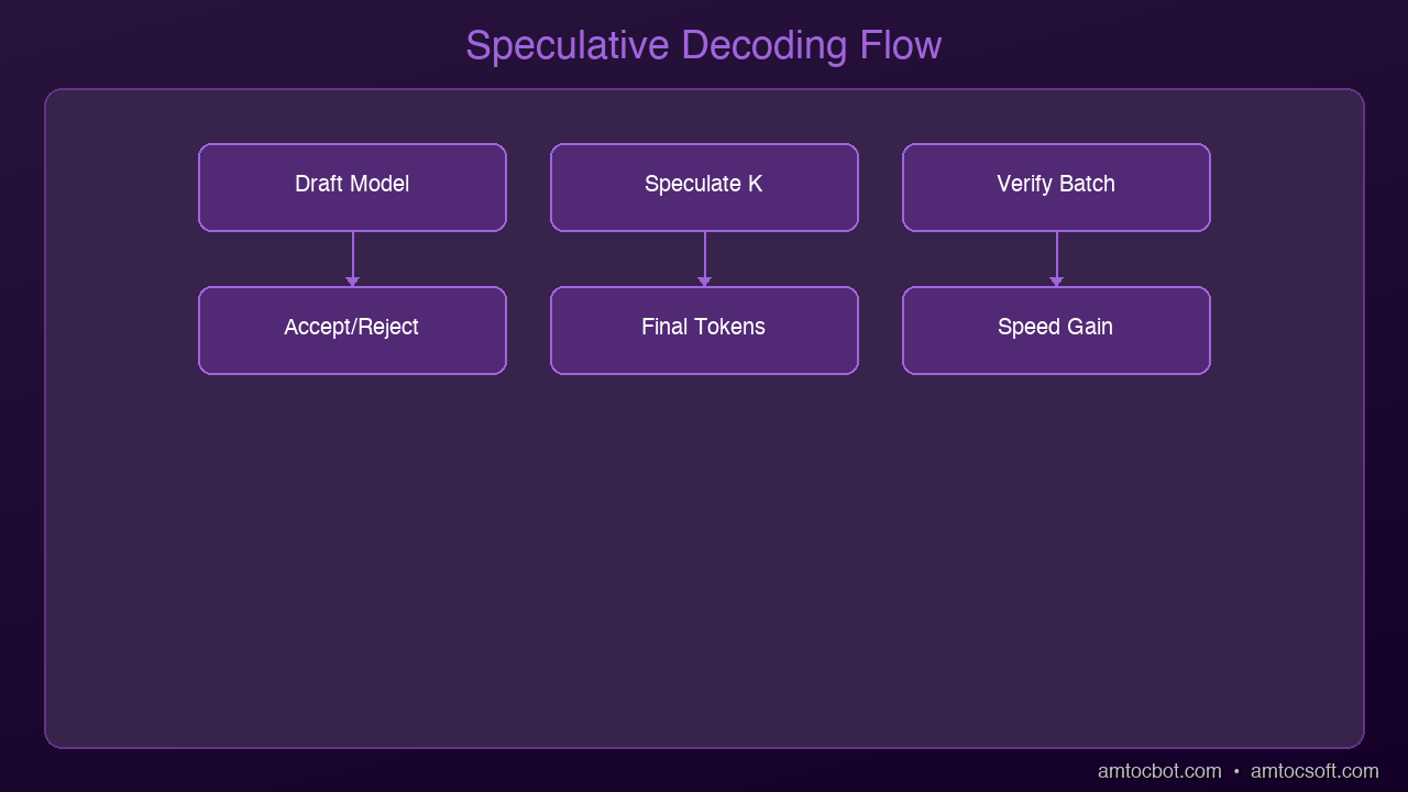
graph LR
  A["Input"] -->|send| B["Draft Model (small/fast)"]
  B -->|"generate N tokens"| C["Large Model verifies all N in parallel"]
  C -->|"accept matches, reject from first mismatch"| D["Output accepted tokens"]
  D -->|repeat| A

The Key Insight

Architecture Diagram

Here's the trick: most tokens are predictable.

When the model generates "The capital of France is", the next token is almost certainly "Paris". You don't need a 70B model to predict that. A tiny 1B model could get it right.

Speculative decoding exploits this by using a small, fast "draft" model to predict multiple tokens ahead, then verifying those predictions with the large model in a single batch.

How It Works

Step 1: Draft Phase
A small model (the "draft model") generates K tokens quickly. Let's say K=5:
- "The" -> "capital" -> "of" -> "France" -> "is" -> "Paris"

This takes milliseconds because the draft model is tiny.

Step 2: Verification Phase
The large model processes all K draft tokens in a single forward pass (parallel verification). It checks each token against what it would have generated.

Step 3: Accept or Reject
- If the large model agrees with a draft token: accept it (free speedup!)
- If it disagrees: reject that token and all subsequent ones, use the large model's token instead

Step 4: Repeat
Start a new draft from wherever the last acceptance ended.

Why This Works

The magic is in the verification step. Normally, the large model processes tokens one-by-one (autoregressive). But checking whether a sequence is correct can be done in parallel -- all K tokens verified in a single pass.

If the draft model has an 80% acceptance rate per token:
- 5 draft tokens -> ~3.2 accepted on average
- Cost: 1 small model pass + 1 large model pass
- Gain: ~3.2 tokens for the cost of ~1.5 tokens
- Net speedup: ~2x

The higher the acceptance rate, the bigger the speedup. For predictable text (code, structured data, common patterns), acceptance rates can exceed 90%, yielding 3x+ speedups.

Real-World Performance

Scenario Draft Model Target Model Acceptance Rate Speedup
Code completion 1B 70B 85-90% 2.5-3x
General chat 1B 70B 70-80% 1.8-2.2x
Creative writing 1B 70B 60-70% 1.5-1.8x
Technical docs 1B 70B 80-85% 2.2-2.8x

Creative writing has the lowest acceptance rate because it's inherently less predictable. Code has the highest because programming languages have rigid syntax.

The Zero Quality Loss Guarantee

This is the critical point: speculative decoding produces mathematically identical output to running the large model alone. It's not an approximation. The verification step guarantees that every accepted token matches what the large model would have generated.

You're not trading quality for speed. You're exploiting the fact that verification is cheaper than generation.

Implementation in Practice

With vLLM (Production)

from vllm import LLM

llm = LLM(
    model="meta-llama/Llama-3.2-70B",
    speculative_model="meta-llama/Llama-3.2-1B",
    num_speculative_tokens=5
)

With llama.cpp (Local)

./main -m llama-70b-q4.gguf \
  --draft-model llama-1b-q8.gguf \
  --draft-max 8 \
  --draft-min 2

Self-Speculative Decoding

Some newer approaches skip the draft model entirely. They use early exit from the large model's own layers as the "draft." Layers 1-8 of a 80-layer model make a quick prediction, and the full 80 layers verify. Same principle, no extra model needed.

2026 Update: EAGLE-3 and Beyond

The speculative decoding landscape has evolved rapidly:

EAGLE-3 achieves 3.0-6.5x speedup over vanilla autoregressive generation -- a 20-40% improvement over EAGLE-2. It fuses information from multiple model layers (not just the top layer) and uses training-time testing to simulate inference conditions during draft model training.

Speculative Speculative Decoding (SSD), published at ICLR 2026, achieves up to 5x over autoregressive and 2x over standard speculative decoding by applying the speculative principle recursively.

Self-speculative decoding is now built into vLLM and SGLang, using early exit from the model's own layers as the draft mechanism -- no separate draft model needed at all.

The trajectory is clear: speculative decoding is moving from "nice optimization" to "table stakes for any serious deployment."

When to Use Speculative Decoding

Great fit:
- Single-user interactive applications (chatbots, coding assistants)
- Latency-sensitive deployments
- GPU memory is available for both models
- Predictable output domains (code, structured data)

Not ideal:
- High-throughput batch processing (batching already saturates the GPU)
- Very short outputs (overhead isn't amortized)
- When GPU memory is too tight for two models
- Extremely creative/diverse outputs (low acceptance rate)

The Bigger Picture

Speculative decoding is part of a broader trend: making inference smarter rather than just making models bigger. Other techniques in this family:

  • KV-cache optimization: Reuse computation across tokens
  • Continuous batching: Process multiple requests simultaneously
  • Flash Attention: Faster attention computation through memory-efficient algorithms
  • Quantization: Reduce model size (covered in our previous post)

Combined, these techniques can make a single GPU serve 10x more users than naive inference. The models aren't getting smaller -- we're just getting dramatically better at running them.


Next: Production AI deployment -- how to serve models to thousands of users with vLLM, TGI, and Triton.

Sources & References:
1. Leviathan et al. — "Fast Inference from Transformers via Speculative Decoding" (2023) — https://arxiv.org/abs/2211.17192
2. Chen et al. — "Accelerating Large Language Model Decoding with Speculative Sampling" (2023) — https://arxiv.org/abs/2302.01318
3. Li et al. — "EAGLE: Speculative Sampling Requires Rethinking Feature Uncertainty" (2024) — https://arxiv.org/abs/2401.15077


About the Author

Toc Am

Founder of AmtocSoft. Writing practical deep-dives on AI engineering, cloud architecture, and developer tooling. Previously built backend systems at scale. Reviews every post published under this byline.

LinkedIn X / Twitter

Published: 2026-04-05 · Written with AI assistance, reviewed by Toc Am.

Get These In Your Inbox

Weekly deep-dives on AI engineering, no fluff. Join the newsletter →

Subscribe (free)

Or grab the book ($39, ~100 pages) · Buy me a coffee

Buy Me a Coffee · 🔔 YouTube · 💼 LinkedIn · 🐦 X/Twitter
Sunday, April 5, 2026

Edge AI: Running Language Models on Phones and IoT Devices

Edge AI Hero

Edge AI: Running Language Models on Phones and IoT Devices

Your phone has more compute power than the servers that trained GPT-2. So why are we still sending every AI request to the cloud?

Edge AI is changing that. In 2026, language models run directly on phones, tablets, laptops, and even embedded devices -- no internet required. Here's how it works and why it matters.

Why Edge AI Matters

Privacy: Your data never leaves your device. Medical questions, financial queries, personal messages -- processed locally, seen by no one.

Latency: No network round-trip. Responses start in milliseconds, not seconds. Critical for real-time applications like voice assistants and AR.

Cost: No API fees. No cloud compute bills. Once the model is on the device, inference is free.

Availability: Works offline. In airplanes, remote areas, or when your cloud provider has an outage.

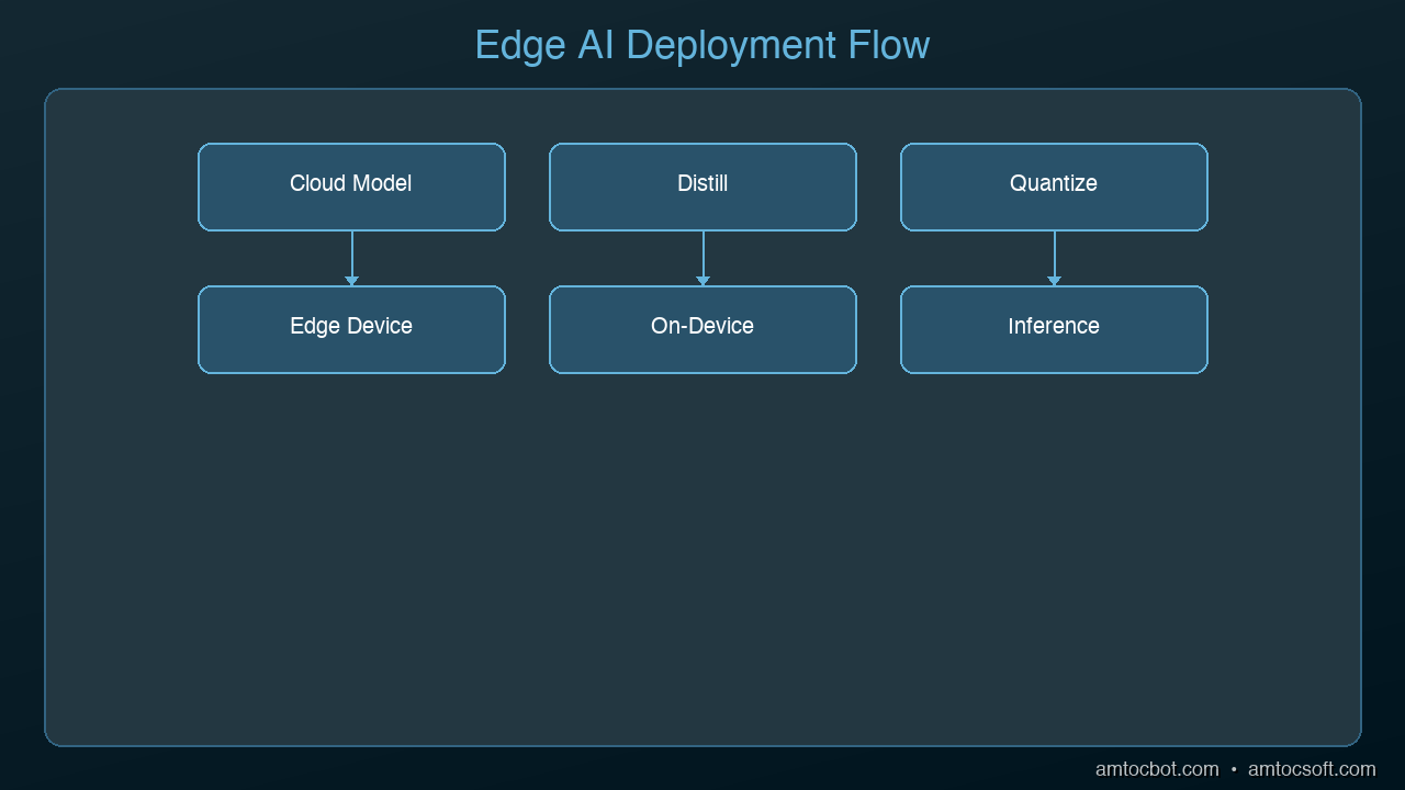
graph LR
  A["Cloud Model"] -->|"quantize & optimize"| B["Convert to Edge Format"]
  B -->|"CoreML / TFLite / ONNX"| C["Deploy to Device"]
  C --> D["On-Device Inference"]
  D --> E["No Internet Needed"]

What's Possible Today

Architecture Diagram

Phones (2026)

Modern smartphones are surprisingly capable AI devices:

  • iPhone 16 Pro: 16 GB unified memory, Apple Neural Engine (38 TOPS). Runs a 3B parameter model at ~15 tokens/second
  • Samsung Galaxy S26: 12 GB RAM, Snapdragon 8 Gen 4 NPU. Runs Gemma 2B at ~20 tokens/second
  • Google Pixel 10: 12 GB RAM, Tensor G5 with dedicated AI core. Runs Gemini Nano natively

These devices comfortably run 1-3B parameter models. With aggressive quantization (Q2-Q4), you can squeeze in a 7B model, though response times slow down.

Laptops (The Sweet Spot)

Apple Silicon Macs have become the default local AI development platform:

  • MacBook Air M3 (24 GB): Runs 7B Q4 at 30+ tokens/sec, 13B Q4 at 15 tokens/sec
  • MacBook Pro M4 Max (128 GB): Runs 70B Q4 at 20+ tokens/sec
  • Framework Laptop (32 GB, Intel/AMD): Runs 7B Q4 at 15-20 tokens/sec via llama.cpp

The Apple MLX framework deserves special mention. It's designed specifically for Apple Silicon's unified memory architecture, delivering 20-40% better performance than generic implementations.

IoT and Embedded

The frontier of edge AI:

  • Raspberry Pi 5 (8 GB): Runs TinyLlama 1.1B at ~3 tokens/sec. Slow, but it works
  • NVIDIA Jetson Orin Nano: 8 GB GPU memory, runs 3B models at 10+ tokens/sec. Perfect for robotics
  • Coral Edge TPU: Specialized for inference, runs small quantized models for classification and simple generation

The Edge AI Stack

Apple Ecosystem: MLX

MLX is Apple's machine learning framework optimized for Apple Silicon. Key advantages:

  • Leverages unified memory (no CPU-to-GPU data copying)
  • Lazy evaluation for memory efficiency
  • NumPy-like API for Python developers
  • Growing model ecosystem on Hugging Face
import mlx.core as mx
from mlx_lm import load, generate

model, tokenizer = load("mlx-community/Llama-3.2-3B-Instruct-4bit")
response = generate(model, tokenizer, prompt="Explain edge AI", max_tokens=200)

Cross-Platform: llama.cpp

llama.cpp runs everywhere -- literally. It's written in pure C/C++ with optional acceleration for:

  • Apple Metal (Mac/iOS)
  • CUDA (NVIDIA GPUs)
  • Vulkan (AMD GPUs, Android)
  • OpenCL (broader GPU support)
  • CPU with SIMD optimizations (AVX2, NEON)

This makes it the go-to choice for cross-platform edge deployment.

Android: MediaPipe LLM

Google's MediaPipe now includes an LLM inference API for Android. It handles model loading, quantization, and hardware acceleration through a simple API:

val llmInference = LlmInference.createFromOptions(context, options)
val response = llmInference.generateResponse("What is edge AI?")

Optimization Techniques for Edge

Running models on constrained devices requires aggressive optimization:

1. Aggressive Quantization

Edge devices benefit most from Q2-Q4 quantization. The quality trade-off is worth it when the alternative is "doesn't fit in memory at all."

2. Knowledge Distillation

Train a small model (1-3B) to mimic a large model (70B). The small model captures 80-90% of the large model's capability at 1/20th the size. This is how Apple Intelligence and Google's on-device models are built.

3. Pruning

Remove unnecessary neurons and connections. Structured pruning can reduce model size by 30-50% with minimal quality loss. Unstructured pruning goes further but requires hardware support.

4. Model Architecture Optimization

Newer architectures designed for edge:
- Gemma 2B: Google's compact model designed for on-device use
- Phi-3 Mini: Microsoft's 3.8B model that punches above its weight
- TinyLlama: 1.1B model trained on 3 trillion tokens -- tiny but capable

5. KV-Cache Compression

On memory-constrained devices, the KV-cache (which grows with context length) is often the bottleneck. Techniques like sliding window attention and grouped-query attention reduce cache size by 4-8x.

Use Cases in Production

Smart Home Assistants: Process voice commands locally. No cloud dependency, instant responses, complete privacy.

Healthcare: Medical devices that analyze patient data on-device. HIPAA compliance is simpler when data never leaves the device.

Automotive: In-car AI for navigation, voice control, and driver assistance. Works in tunnels and dead zones.

Industrial IoT: Predictive maintenance on factory floors. Analyze sensor data locally, alert only when needed.

Education: Offline tutoring apps for students without reliable internet. Especially impactful in developing regions.

The Trade-offs

Edge AI isn't always the right choice:

Factor Edge Cloud
Model Size 1-7B Unlimited
Response Quality Good Best
Latency <100ms 200ms-2s
Privacy Complete Depends on provider
Cost per Query Free $0.001-0.01
Offline Support Yes No
Updates Manual Automatic

The emerging pattern is hybrid: use edge AI for simple, latency-sensitive, or privacy-critical tasks, and fall back to cloud for complex reasoning that requires larger models.

Getting Started

The fastest path to edge AI:

  1. Mac users: Install Ollama, run ollama run llama3.2:3b
  2. Mobile developers: Try MediaPipe LLM (Android) or Core ML (iOS)
  3. IoT: Start with a Jetson Orin Nano and llama.cpp
  4. Web: Use WebLLM to run models directly in the browser via WebGPU

Edge AI isn't a future technology. It's a today technology that's getting better every month. The models are getting smaller, the hardware is getting faster, and the tools are getting simpler.


Next: Putting it all together -- a complete guide to choosing your AI deployment strategy from development to production.

Sources & References:
1. Apple — "Core ML Documentation" — https://developer.apple.com/documentation/coreml
2. Google — "MediaPipe Solutions" — https://ai.google.dev/edge/mediapipe/solutions/guide
3. ONNX Runtime — "Mobile and Edge Deployment" — https://onnxruntime.ai/


About the Author

Toc Am

Founder of AmtocSoft. Writing practical deep-dives on AI engineering, cloud architecture, and developer tooling. Previously built backend systems at scale. Reviews every post published under this byline.

LinkedIn X / Twitter

Published: 2026-04-05 · Written with AI assistance, reviewed by Toc Am.

Get These In Your Inbox

Weekly deep-dives on AI engineering, no fluff. Join the newsletter →

Subscribe (free)

Or grab the book ($39, ~100 pages) · Buy me a coffee

Buy Me a Coffee · 🔔 YouTube · 💼 LinkedIn · 🐦 X/Twitter
Speculative Decoding: How to Make LLMs 2-3x Faster for Free

Speculative Decoding: How to Make LLMs 2-3x Faster for Free What if you could make your LLM generate text 2-3x faster without changing the model, without losing any quality, and without buying better hardware? That's the promise of speculative decoding -- and it actually delivers. The Speed Problem LLMs generate text one token at a time. Each token requires a full forward pass through the entire model. For a 70B model, that means: - 70 billion multiply-and-add operations per token - At 30 tokens per second, generating a 500-word response takes ~50 seconds - The GPU sits idle for much of this time, waiting for memory transfers The bottleneck isn't compute -- it's memory bandwidth. The GPU can do math faster than it can load model weights from memory. This is called being "memory-bound." The Key Insight Here's the trick: most tokens are predictable. When the model generates "The capital of France is", the next token is almost certainly "Paris". You don't need a 70B model to predict that. A tiny 1B model could get it right. Speculative decoding exploits this by using a small, fast "draft" model to predict multiple tokens ahead, then verifying those predictions with the large model in a single batch. How It Works Step 1: Draft Phase A small model (the "draft model") generates K tokens quickly. Let's say K=5: "The" -> "capital" -> "of" -> "France" -> "is" -> "Paris" This takes milliseconds because the draft model is tiny. Step 2: Verification Phase The large model processes all K draft tokens in a single forward pass (parallel verification). It checks each token against what it would have generated. Step 3: Accept or Reject - If the large model agrees with a draft token: accept it (free speedup!) - If it disagrees: reject that token and all subsequent ones, use the large model's token instead Step 4: Repeat Start a new draft from wherever the last acceptance ended. Why This Works The magic is in the verification step. Normally, the large model processes tokens one-by-one (autoregressive). But checking whether a sequence is correct can be done in parallel -- all K tokens verified in a single pass. If the draft model has an 80% acceptance rate per token: - 5 draft tokens -> ~3.2 accepted on average - Cost: 1 small model pass + 1 large model pass - Gain: ~3.2 tokens for the cost of ~1.5 tokens - Net speedup: ~2x The higher the acceptance rate, the bigger the speedup. For predictable text (code, structured data, common patterns), acceptance rates can exceed 90%, yielding 3x+ speedups. Real-World Performance Code completion: 1B draft, 70B target, 85-90% acceptance, 2.5-3x speedup General chat: 1B draft, 70B target, 70-80% acceptance, 1.8-2.2x speedup Creative writing: 1B draft, 70B target, 60-70% acceptance, 1.5-1.8x speedup Technical docs: 1B draft, 70B target, 80-85% acceptance, 2.2-2.8x speedup Creative writing has the lowest acceptance rate because it's inherently less predictable. Code has the highest because programming languages have rigid syntax. The Zero Quality Loss Guarantee This is the critical point: speculative decoding produces mathematically identical output to running the large model alone. It's not an approximation. The verification step guarantees that every accepted token matches what the large model would have generated. You're not trading quality for speed. You're exploiting the fact that verification is cheaper than generation. Implementation in Practice With vLLM (Production): from vllm import LLM llm = LLM( model="meta-llama/Llama-3.2-70B", speculative_model="meta-llama/Llama-3.2-1B", num_speculative_tokens=5 ) With llama.cpp (Local): ./main -m llama-70b-q4.gguf --draft-model llama-1b-q8.gguf --draft-max 8 --draft-min 2 Self-Speculative Decoding Some newer approaches skip the draft model entirely. They use early exit from the large model's own layers as the "draft." Layers 1-8 of an 80-layer model make a quick prediction, and the full 80 layers verify. Same principle, no extra model needed. 2026 Update: EAGLE-3 and Beyond The speculative decoding landscape has evolved rapidly: EAGLE-3 achieves 3.0-6.5x speedup over vanilla autoregressive generation -- a 20-40% improvement over EAGLE-2. It fuses information from multiple model layers (not just the top layer) and uses training-time testing to simulate inference conditions during draft model training. Speculative Speculative Decoding (SSD), published at ICLR 2026, achieves up to 5x over autoregressive and 2x over standard speculative decoding by applying the speculative principle recursively. Self-speculative decoding is now built into vLLM and SGLang, using early exit from the model's own layers as the draft mechanism -- no separate draft model needed at all. The trajectory is clear: speculative decoding is moving from "nice optimization" to "table stakes for any serious deployment." When to Use Speculative Decoding Great fit: - Single-user interactive applications (chatbots, coding assistants) - Latency-sensitive deployments - GPU memory is available for both models - Predictable output domains (code, structured data) Not ideal: - High-throughput batch processing (batching already saturates the GPU) - Very short outputs (overhead isn't amortized) - When GPU memory is too tight for two models - Extremely creative/diverse outputs (low acceptance rate) The Bigger Picture Speculative decoding is part of a broader trend: making inference smarter rather than just making models bigger. Other techniques in this family: - KV-cache optimization: Reuse computation across tokens - Continuous batching: Process multiple requests simultaneously - Flash Attention: Faster attention computation through memory-efficient algorithms - Quantization: Reduce model size (covered in our previous post) Combined, these techniques can make a single GPU serve 10x more users than naive inference. The models aren't getting smaller -- we're just getting dramatically better at running them. Next: Production AI deployment -- how to serve models to thousands of users with vLLM, TGI, and Triton.

Attention Is All You Need, Explained Simply

We published a plain-language walkthrough of the 2017 transformer paper — queries, keys, values, multi-head attention, and why no-recurrence...