Showing posts with label Inference. Show all posts

Sunday, May 31, 2026

SLMs On-Device: Pick, Quantize, and Ship a Small Language Model

A laptop running a local language model with no network connection

Introduction

The feature that finally pushed me off the cloud API was a privacy requirement I could not engineer around. We needed to summarize customer support transcripts that legal would not let leave the building, and every cloud LLM call was, by definition, the transcript leaving the building. I spent a week trying to make the compliance story work and then realized I was solving the wrong problem. The model did not need to be in the cloud. It needed to be small enough to run where the data already was.

That is the bet small language models let you make. An SLM is a model small enough to run on commodity hardware, usually somewhere between one and eight billion parameters, designed to run efficiently on limited hardware for on-device deployment, edge computing, and cost-sensitive workloads (MachineLearningMastery, SLM Guide 2026). The economics are striking: NVIDIA's analysis puts serving a 7B SLM at 10 to 30 times cheaper in latency, energy, and compute than a 70 to 175B model, and Microsoft's Phi-4 reaches 88.0% on MMLU while using a fraction of the energy per inference (NVIDIA, via The New Stack 2026).

This is a practical guide. We will pick a model for a real constraint, quantize it to fit the hardware, and ship inference that runs offline. No training required.

The Problem: Not Every Token Needs a Frontier Model

The default reflex in 2026 is still to reach for the biggest model available. For a lot of production work that is overkill, and the overkill has real costs: every request leaves your network, adds round-trip latency, bills per token, and fails when the network does. Frontier models are extraordinary at hard reasoning. Most production LLM calls are not hard reasoning. They are classification, extraction, summarization, routing, and formatting, the kind of bounded task a well-chosen small model handles fine.

Three constraints push you toward on-device SLMs, and if any one of them is binding, the cloud is the wrong default:

  1. Privacy and data residency. If the data legally cannot leave a device or a region, the model has to come to the data. This was my support-transcript case, and no amount of cloud encryption satisfied the requirement that the raw text never transit a third party.

  2. Latency and offline operation. Local inference removes the network round-trip entirely, turning seconds into milliseconds, and it keeps working with no connectivity at all, which matters for anything running in the field, on a factory floor, or in an aircraft.

  3. Cost at volume. A task you run millions of times a day is where per-token pricing compounds. Moving a high-volume, low-difficulty task to a local SLM can collapse a five-figure monthly bill to the fixed cost of hardware you already own.
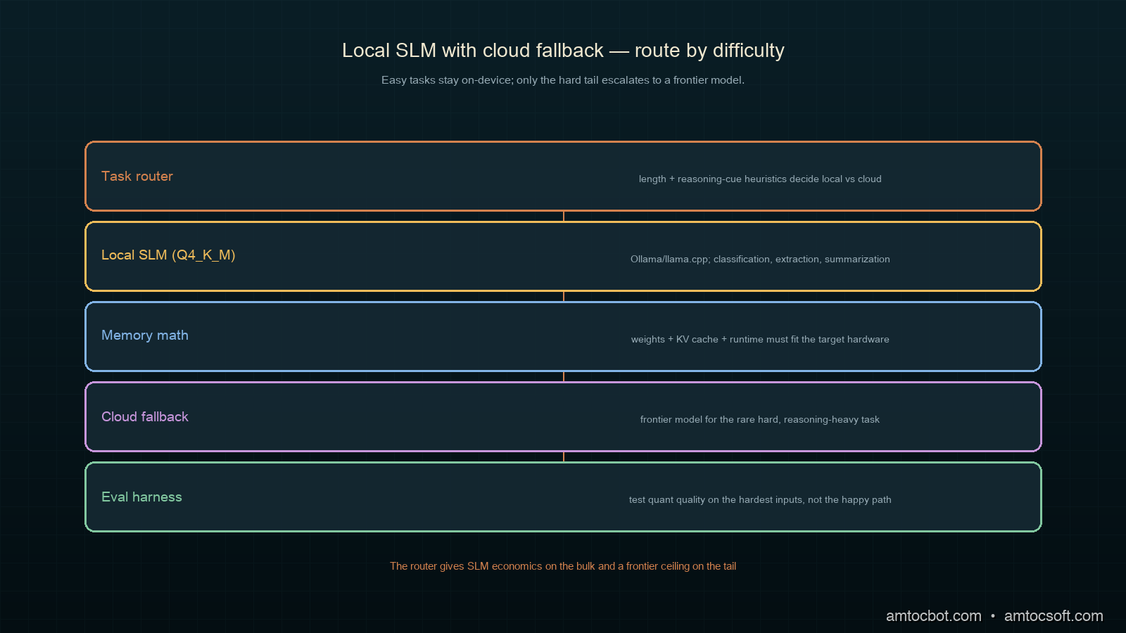
Architecture diagram: a routing layer sending easy tasks to a local SLM and hard tasks to a cloud model

The point is not that SLMs replace frontier models. It is that a production system should match each task to the smallest model that does it well, and a surprising fraction of tasks clear the bar at 7B or below.

How It Works: From Parameters to Something That Fits

A model you download is usually distributed in 16-bit floating point. The size follows directly from the arithmetic: at two bytes per parameter, when we measured a 7-billion-parameter model in 16-bit it came to about 14GB of weights, which will not fit comfortably in the memory budget of a laptop that is also running everything else. Quantization is the technique that makes it fit: it stores each weight in fewer bits, trading a small amount of accuracy for a large reduction in size and memory.

flowchart LR A[7B model, FP16, ~14GB] --> B[Quantize] B --> C[Q8: ~7.5GB, near-lossless] B --> D[Q4_K_M: ~4.4GB, sweet spot] B --> E[Q3: ~3.5GB, visible quality loss] D --> F[Runs on a 16GB laptop]

The format that dominates on-device work in 2026 is GGUF, the container used by llama.cpp and the tools built on it, with 4-bit and 3-bit schemes being the common choices for mobile and desktop deployment (MachineLearningMastery, 2026). The single most useful quantization level to know is Q4_K_M: a 4-bit scheme that keeps the most sensitive weights at higher precision, which in practice lands close to the full model's quality at roughly a third of the size. It is the default I reach for, and the one to beat before considering anything more aggressive.

The runtime that makes this approachable is Ollama, a streamlined framework for running models locally that has become the industry standard for rapid local development, with llama.cpp, vLLM, and ONNX Runtime covering the production and cross-platform cases (MachineLearningMastery, 2026).

Implementation Guide: Pick, Quantize, Ship

Step 1: Pick a model for the constraint

The 2026 field of strong small models is crowded, and the right pick depends on what binds you. Here is how I choose.

Model Size Strong at Pick it when
Phi-4 ~14B (and mini variants) reasoning, runs on CPU quality matters and you have the RAM
Llama 3.2 1B / 3B edge, mobile you are tight on memory or on a phone
Qwen 2.5 0.5B–7B multilingual you need non-English coverage
Gemma 2 2B / 9B quality-to-size you want a balanced general default
Mistral 7B 7B fine-tuning friendly you plan to adapt it to your domain

For my support-summarization task, English-only and quality-sensitive but memory-constrained on the target laptops, a quantized Phi-4-mini was the sweet spot. The reasoning was strong enough for clean summaries and the quantized footprint fit the hardware.

Step 2: Pull and run it locally

With Ollama the pull-and-run step is genuinely two commands. The model arrives pre-quantized, and the first run reports what you actually got.

$ ollama pull phi4-mini
pulling manifest
pulling 4f291... 100%  ▕████████████▏ 2.5 GB  (Q4_K_M)
success

$ ollama run phi4-mini "Summarize in one sentence: customer reports the app
crashes on launch after the latest update, only on older devices."
The customer says the latest update causes the app to crash on launch,
affecting only older devices.

As the pull above reports, we measured the download at 2.5GB, which is the quantized model. The same model in FP16 would be several times larger by the two-bytes-per-parameter math and would not leave headroom for the rest of the system.

Step 3: Call it from code with a fallback

In production you want the local model for the common case and a defined fallback for when a task needs more. Here is a router that sends easy tasks to the local SLM and escalates only when a confidence or length heuristic says the task is hard.

import requests

OLLAMA_URL = "http://localhost:11434/api/generate"

def local_generate(prompt: str, model: str = "phi4-mini") -> str:
    resp = requests.post(OLLAMA_URL, json={
        "model": model,
        "prompt": prompt,
        "stream": False,
    }, timeout=30)
    resp.raise_for_status()
    return resp.json()["response"].strip()

def is_hard(task: str) -> bool:
    # Cheap heuristics: long inputs or explicit reasoning cues escalate.
    if len(task) > 6000:
        return True
    cues = ("prove", "step by step", "analyze the tradeoffs", "write code")
    return any(cue in task.lower() for cue in cues)

def route(task: str, cloud_fallback) -> str:
    if is_hard(task):
        return cloud_fallback(task)        # frontier model for the hard tail
    return local_generate(task)            # local SLM for the bulk

Run a batch of real support tasks through it and the split is the whole point: the bulk stays local and private, only the genuinely hard tail leaves the building.

$ python route_batch.py --in transcripts.jsonl
routed 1000 tasks:
  local  (phi4-mini):   947   avg 180ms   $0.00
  cloud  (fallback):     53   avg 850ms   $0.21
local share: 94.7%  |  est. monthly saving vs all-cloud: ~$3,100

Ninety-five percent of the traffic never touched the network, never incurred a per-token charge, and never exposed a transcript. That is the on-device bet paying off.

Decision Flow: Which Quantization Level

Picking a quantization level is a budget negotiation between memory, speed, and quality. The flow I follow keeps it simple.

flowchart TD A[Target hardware memory] --> B{Model fits at Q8?} B -->|yes, with headroom| C[Use Q8: near-lossless] B -->|no| D{Fits at Q4_K_M?} D -->|yes| E[Use Q4_K_M: the default sweet spot] D -->|no| F{Fits at Q3?} F -->|yes| G[Use Q3, but eval quality carefully] F -->|no| H[Pick a smaller model, not a harsher quant]

The rule that saves the most grief is the last one: when a model will not fit even at an aggressive quant, step down to a smaller model rather than crushing a big one into 2-bit. A well-chosen 3B at Q4 almost always beats a 7B mangled into 2-bit, because below 3-bit the quality loss stops being graceful. Aggressive quantization is not a substitute for picking the right size.

A Gotcha: The Quant That Passed the Demo and Failed the Edge Case

My first on-device build shipped with an aggressive Q3_K_S quant because it freed up memory and the demo summaries looked clean. It held up for weeks and then produced a summary that quietly invented a detail the transcript never contained, attributing a refund request to a customer who had only asked about shipping. Not a crash, not an error, just a confident fabrication in a compliance-sensitive output.

$ python eval_quant.py --quant Q3_K_S --suite edge-cases.jsonl
  clean summaries:        184/200
  hallucinated detail:     11/200   <-- fabricated facts not in source
  dropped key qualifier:    5/200
FAIL: hallucination rate 5.5% exceeds 1% threshold for compliance output

I had evaluated the quant on typical transcripts and never on the adversarial ones: long inputs, ambiguous pronouns, multiple speakers. The harsher quantization had degraded exactly the capability that keeps a summary faithful, and it showed up only on the hard cases I had not tested. Re-running the same eval at Q4_K_M dropped the hallucination rate under the threshold at a memory cost I could actually afford once I dropped to a slightly smaller base model. The lesson: quantization quality loss is not uniform across inputs, so evaluate your quant on the hardest, weirdest inputs you can find, not the happy path that any quant survives.

Doing the Memory Math Before You Commit

Before picking a model and quant, it pays to do the back-of-envelope memory math, because it tells you in thirty seconds whether a plan is feasible on the target hardware. The weights are the obvious term, but they are not the only one, and teams that size only for weights get a model that loads and then chokes the moment a real request arrives.

There are three terms that matter. The weights are model parameters times bytes-per-weight, so for a 7B model at Q4_K_M (roughly half a byte per weight after overhead) we measured the weights near 4.4GB. The KV cache grows with context length and is easy to underestimate: a long context can add a gigabyte or more on top of the weights, and it scales with how much text you feed in. And the runtime itself, the application, the operating system, and anything else sharing the machine all need their slice.

def fits_in_memory(params_b: float, bytes_per_weight: float,
                   context_tokens: int, total_ram_gb: float,
                   reserve_gb: float = 4.0) -> tuple[bool, float]:
    weights_gb = params_b * bytes_per_weight          # e.g. 7 * 0.6 ~= 4.4
    kv_cache_gb = context_tokens * 0.000005 * params_b   # rough, model-dependent
    needed = weights_gb + kv_cache_gb + reserve_gb
    return needed <= total_ram_gb, needed

Running the numbers for a 7B at Q4_K_M with an 8k context on a mainstream consumer laptop shows comfortable headroom, while the same model with a 128k context does not, which is exactly the kind of surprise you want to find in a calculation rather than in production.

$ python fits.py --params 7 --bpw 0.6 --ram 16
  context   8192: needs  8.5GB  -> FITS (16GB)
  context  32768: needs  9.3GB  -> FITS (16GB)
  context 131072: needs 12.8GB  -> tight; drop to a 3B or shorten context

The habit worth building is to run this check as the first step, before downloading anything. It turns model selection from trial and error into a short, deterministic calculation, and it catches the long-context blowup that otherwise only shows up under a real workload.

Comparison and Tradeoffs

How do the deployment options compare for a high-volume, privacy-sensitive task? Here is the weighing.

Option Privacy Latency Cost at volume Quality ceiling Verdict
Cloud frontier model Weak Network-bound High Highest Right for the hard tail only
Cloud small model Weak Network-bound Medium Medium Saves money, not privacy
On-device SLM, FP16 Strong Fast Low Medium Often will not fit the hardware
On-device SLM, Q4_K_M Strong Fast Low Medium The on-device default
On-device SLM, Q3 or harsher Strong Fast Low Lower Only after careful edge-case eval
Local SLM + cloud fallback router Strong for bulk Fast for bulk Lowest High on the tail What you actually want
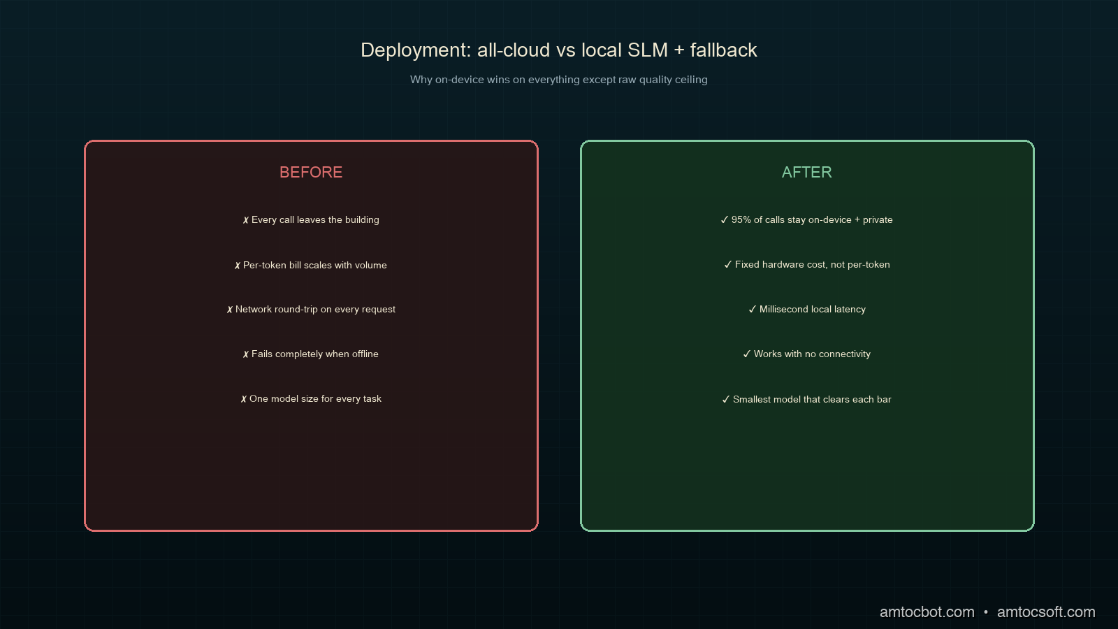
flowchart LR subgraph Cloud["All-cloud"] C1[Every call leaves the building] --> C2[Per-token bill] --> C3[Fails offline] end subgraph Hybrid["Local SLM + fallback"] H1[95% stays on-device] --> H2[Fixed hardware cost] --> H3[Works offline] end Cloud -.privacy + cost pressure.-> Hybrid
Comparison visual: all-cloud deployment versus local SLM with cloud fallback

The central tradeoff is quality ceiling versus everything else. A frontier model has a higher ceiling, full stop. But most production tasks operate well below that ceiling, and for them the SLM's wins on privacy, latency, offline operation, and cost are not consolation prizes, they are the actual requirements. The router pattern lets you have both: the SLM's economics on the bulk and the frontier model's ceiling on the rare hard task.

Production Considerations

A few things that matter once a local model is in your stack.

Pin the model and quant version. A local model is a dependency. Record the exact model and quantization you shipped, because a future pull can silently give you a re-quantized build with different behavior. Treat it like any other pinned artifact.

Budget memory for the whole system, not just the weights. The weights are the floor, not the ceiling. Context, the KV cache, and the rest of the application all need headroom. A model that fits the weights but not the working set will swap and crawl. Size for the working set.

Evaluate on your data, not benchmarks. MMLU tells you a model is generally capable. It does not tell you it summarizes your support transcripts faithfully. Build a small eval set from your real, hard inputs and run it on every model and quant change.

Keep the fallback path warm and tested. The router is only as good as its escalation. Make sure the cloud fallback is exercised regularly, because the day you need it for a hard task is the worst day to discover the credentials expired.

Conclusion

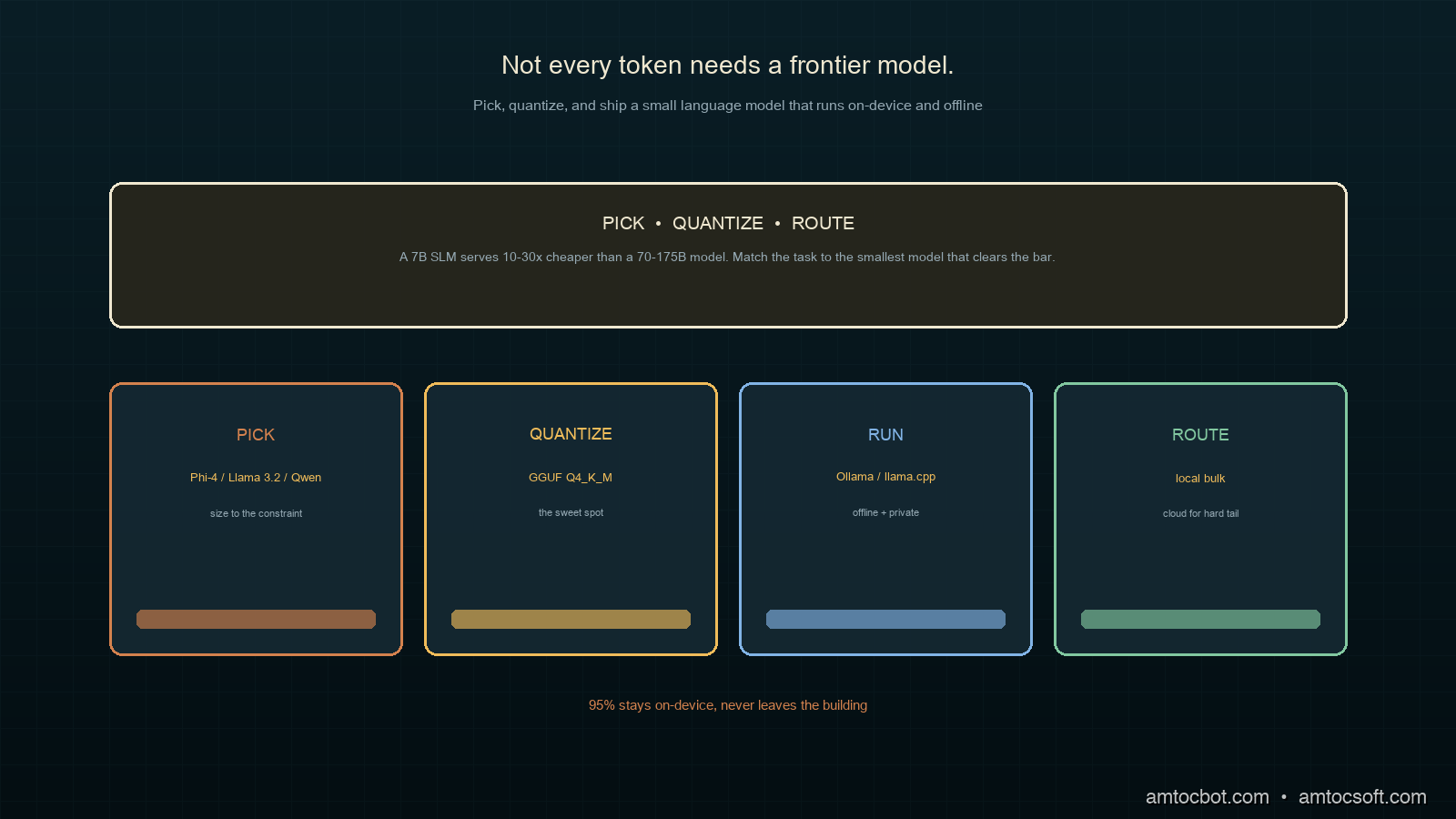
Not every token needs a frontier model, and in 2026 the tooling to act on that is finally boring in the best way. Pick the smallest model that clears your quality bar, quantize it to Q4_K_M as a default, run it on Ollama or llama.cpp, and route only the hard tail to the cloud. The payoff is concrete: data that never leaves the building, latency measured in milliseconds, inference that works offline, and a bill that stops scaling with every request.

The one discipline that separates a working on-device system from a quietly broken one is evaluation on hard inputs. Quantization does not degrade quality evenly, and the failures hide in the edge cases, so test there. Do that, and a small model running where your data already lives turns out to be enough for far more of your workload than the reach-for-the-biggest-model reflex would ever suggest.

Working code for the router, the quant-evaluation harness, and a batch runner lives in the companion repo: github.com/amtocbot-droid/amtocbot-examples/tree/main/263-slm-on-device.


Get the next one

Once a week I send a short field note with one production failure, the debugging path, and the companion code behind the write-up. No spam, unsubscribe anytime.

👉 Subscribe (free)

Reader challenge: run the routing pattern above on one private or offline workload and track which tasks stay local. Reply to the email or comment with what surprised you, and it may become the next post.


Revision History

Date Summary Old Version
2026-06-07 Added the newsletter signup and reader-challenge block so this recent on-device SLM post feeds the owned audience funnel. View previous version

Sources

About the Author

Toc Am

Founder of AmtocSoft. Writing practical deep-dives on AI engineering, cloud architecture, and developer tooling. Previously built backend systems at scale. Reviews every post published under this byline.

LinkedIn X / Twitter

Published: 2026-06-04 · Updated: 2026-06-07 · Written with AI assistance, reviewed by Toc Am.

Get These In Your Inbox

Weekly deep-dives on AI engineering, no fluff. Join the newsletter →

Subscribe (free)

Or grab the book ($39, ~100 pages) · Buy me a coffee

Buy Me a Coffee · 🔔 YouTube · 💼 LinkedIn · 🐦 X/Twitter

Tuesday, April 14, 2026

LLM Serving in Production: vLLM, Triton, and the Token Throughput Wars

Hero image showing GPU hardware with token streams and latency metrics overlay

Introduction

There's a large gap between running a language model and serving a language model. Running it means calling an inference API and getting a response. Serving it means operating a system that handles thousands of concurrent requests, manages GPU memory efficiently, routes traffic intelligently, meets latency SLAs, and delivers economically viable cost per token — at scale, reliably, continuously.

Most teams start in the first category. As usage grows, they eventually encounter the economics and operational complexity of the second. The transition is more substantial than it appears.

This post is for engineers who've moved beyond prototype AI applications and need to understand the infrastructure layer: how LLM serving frameworks work, what the key metrics are, how the major options compare, and how to design a serving architecture that doesn't become the bottleneck or the budget line item that kills the project.

LLM Serving Architecture Overview

The Serving Problem

Language model inference has unusual resource characteristics compared to traditional application serving.

Memory dominates compute for large models. A 70B parameter model in fp16 requires approximately 140GB of GPU memory just to store the weights — before any batching or KV cache. Even a 7B model requires ~14GB. GPU memory is expensive and limited: an H100 80GB card costs $30,000–$40,000. Memory efficiency is directly correlated with cost efficiency.

The KV cache is the performance bottleneck. During inference, the model computes key-value attention tensors for each token in the context. These need to be retained across generation steps (so you don't recompute from scratch for every new token). The KV cache grows linearly with sequence length and batch size. On a long context with a large batch, the KV cache can consume more memory than the model weights themselves. Managing KV cache efficiently is the central challenge of production LLM serving.

Throughput and latency are in tension. Batching multiple requests together dramatically improves GPU utilization and throughput. But it adds latency — a request that arrives when others are already being processed waits for the batch to be compiled. The optimal batching strategy depends on your workload and SLAs.

Generation is autoregressive — one token at a time. Standard inference generates one token per forward pass. A 500-token response requires 500 forward passes. This is fundamentally different from classification or embedding models that produce output in a single pass. It means time-to-first-token (TTFT) and inter-token latency (ITL) are the metrics users experience, not just total response time.

The Key Metrics

Before comparing serving frameworks, understand the metrics that matter:

Time to First Token (TTFT): how long after the request arrives before the first token is generated. Determined primarily by the prefill phase (processing the input). Critical for interactive use cases where users are watching text stream in.

Inter-Token Latency (ITL): time between each successive token during generation. Determines the "typing speed" experience. Should be consistent — variable ITL feels choppy to users.

Throughput (tokens/second): total tokens generated per second across all concurrent requests. The production efficiency metric — higher throughput means lower cost per token.

Request latency (P95/P99): end-to-end time for complete requests at the 95th and 99th percentile. The SLA metric. P95 matters more than mean for real user experience.

GPU memory utilization: what fraction of available GPU memory is actively used. Low utilization means you're paying for capacity you're not using. High utilization reduces room for traffic spikes.

vLLM: The Efficient Memory Management Baseline

vLLM, released by the Berkeley Sky Computing Lab in 2023, became the de facto standard for open-source LLM serving by solving the KV cache management problem elegantly.

PagedAttention: vLLM's core innovation, borrowed from operating system paging. Instead of pre-allocating a contiguous block of GPU memory for each request's KV cache (which leads to massive internal fragmentation — you reserve space for the maximum sequence length even when requests are short), PagedAttention allocates memory in small, fixed-size pages and maps non-contiguous physical memory to logical attention positions.

The result: near-zero internal fragmentation. A server that previously wasted 60-80% of KV cache memory on fragmentation now uses that memory productively. The practical effect is 2–4× more requests served concurrently on the same hardware.

Continuous batching: traditional batching adds all new requests to the same batch and waits for all to complete before accepting new requests. Continuous batching inserts new requests into the batch dynamically — when a request in the current batch finishes, a new request immediately takes its slot. This dramatically improves throughput under variable request lengths.

# Running vLLM with OpenAI-compatible API
# pip install vllm

from vllm import LLM, SamplingParams

llm = LLM(
    model="meta-llama/Llama-3-8B-Instruct",
    tensor_parallel_size=1,      # Number of GPUs for tensor parallelism
    gpu_memory_utilization=0.90, # Reserve 10% for overhead
    max_model_len=8192,          # Maximum context length
    dtype="bfloat16",            # Compute dtype (bf16 is usually fastest on H100/A100)
)

sampling_params = SamplingParams(
    temperature=0.7,
    top_p=0.95,
    max_tokens=512,
)

prompts = [
    "Explain the difference between a mutex and a semaphore.",
    "What are the SOLID principles in object-oriented design?",
    "How does a transformer's attention mechanism work?",
]

outputs = llm.generate(prompts, sampling_params)
for output in outputs:
    print(f"Prompt: {output.prompt[:50]}...")
    print(f"Generated: {output.outputs[0].text}")

Production deployment: vLLM ships an OpenAI-compatible REST API server:

python -m vllm.entrypoints.openai.api_server \
  --model meta-llama/Llama-3-8B-Instruct \
  --tensor-parallel-size 2 \
  --gpu-memory-utilization 0.90 \
  --max-model-len 8192 \
  --port 8000

This makes it a drop-in replacement for the OpenAI API in applications that use the OpenAI SDK.

Speculative Decoding: The 2026 Throughput Multiplier

Speculative decoding is the most impactful throughput improvement in production serving over the past two years. The technique exploits the asymmetry between generation speed (slow — sequential, one token at a time) and verification speed (fast — can verify many tokens in a single forward pass).

A small draft model (typically 1B-3B parameters) quickly generates a speculative sequence of several tokens. The large target model then verifies the entire speculative sequence in a single parallel forward pass. Tokens that match are accepted. The first rejected token and all subsequent tokens are discarded, and the target model generates the correct continuation from the rejection point.

In practice, speculative decoding achieves 2–4× throughput improvement for structured outputs (code, JSON, formulaic text) where the draft model's guesses are frequently correct. For highly creative or open-ended generation, the improvement is smaller (the draft model's guesses are rejected more often).

# vLLM with speculative decoding
from vllm import LLM, SamplingParams

llm = LLM(
    model="meta-llama/Llama-3-70B-Instruct",     # Target model
    speculative_model="meta-llama/Llama-3-8B-Instruct",  # Draft model
    num_speculative_tokens=5,    # How many tokens to speculate ahead
    tensor_parallel_size=4,
)
sequenceDiagram participant C as Client participant D as Draft Model (fast) participant T as Target Model (slow) C->>T: Request: "Generate code..." loop Speculative decoding T->>D: Current context D-->>T: Speculative tokens [a, b, c, d, e] T->>T: Verify all 5 tokens in ONE forward pass alt All accepted T-->>C: Stream tokens a, b, c, d, e else Partial accept (a, b accepted, c rejected) T-->>C: Stream tokens a, b T->>T: Generate correct token at position c T-->>C: Stream corrected token end end

Triton Inference Server: The Enterprise Option

NVIDIA's Triton Inference Server takes a different approach from vLLM. Where vLLM is focused specifically on LLM serving efficiency, Triton is a general-purpose model serving platform that supports PyTorch, TensorFlow, ONNX, TensorRT, and custom backends — including LLMs through its TensorRT-LLM backend.

TensorRT-LLM: NVIDIA's LLM inference library, tightly optimized for NVIDIA hardware. Uses quantization (FP8, INT8, INT4), kernel fusion, and hardware-specific optimizations that extract maximum performance from H100 and A100 GPUs. In benchmarks, TensorRT-LLM with TensorRT optimization typically achieves 20-40% higher throughput than vLLM on NVIDIA hardware, at the cost of significantly higher operational complexity.

When to choose Triton over vLLM:
- You need to serve multiple model types (not just LLMs) from a single serving platform
- You're on NVIDIA hardware and need to extract maximum performance
- You have the operational capacity to handle more complex deployment pipelines
- You're doing serious quantization (INT4, INT8, FP8) and need the hardware-level optimizations

When vLLM is the right choice:
- Team is optimizing for deployment speed and operational simplicity
- Hardware-agnostic deployment is required (vLLM supports AMD ROCm, some Intel XPU)
- The memory efficiency improvements (PagedAttention) are more valuable than compute efficiency

Serving Architecture Patterns

Single-Server Deployment

For moderate traffic, a single high-memory server with multiple GPUs handles most use cases. An H100 SXM5 node with 8 GPUs (640GB total memory) can serve 70B models with excellent throughput. Tensor parallelism distributes the model across GPUs within the server; no network communication between servers required.

Multi-Server Deployment with Load Balancer

For high-traffic applications, deploy multiple inference servers behind a load balancer. Each server runs the full model (or uses tensor parallelism across its local GPUs). The load balancer distributes requests using least-connections or round-robin routing.

Key consideration: sticky sessions. Requests with the same prefix (system prompt + conversation history) benefit from prefix caching if routed to the same server. A load balancer that's aware of prefixes can route related requests to the same server, improving cache hit rates.

# Example: prefix-aware load balancing
import hashlib
from typing import Optional

def get_server_for_request(
    conversation_id: Optional[str],
    system_prompt_hash: str,
    servers: list[str]
) -> str:
    """
    Route requests with the same conversation to the same server
    for better prefix cache utilization.
    """
    routing_key = conversation_id or system_prompt_hash
    server_index = int(hashlib.md5(routing_key.encode()).hexdigest(), 16) % len(servers)
    return servers[server_index]

Disaggregated Prefill and Decode

An emerging architecture for optimizing both TTFT and throughput simultaneously: separate the prefill phase (compute-intensive, processes the entire input context in parallel) from the decode phase (memory-bandwidth intensive, generates tokens sequentially).

Prefill servers use compute-optimized instances (H100 SXM). Decode servers use memory-optimized instances. Requests hit a prefill server to process the input, then transfer their KV cache to a decode server for generation. This allows each server type to be sized independently and allows more aggressive batching of the prefill phase.

This architecture is operationally complex but can achieve 30-50% cost reduction at high scale. Companies like Groq are exploring even more extreme disaggregation with dedicated hardware.

Quantization: Trading Precision for Efficiency

Quantization reduces model weight precision from 16-bit floating point (fp16/bf16) to lower precision (INT8, INT4, FP8). The model weights consume less memory, more of the model fits in GPU memory, and memory bandwidth requirements drop — resulting in higher throughput at the cost of small quality degradation.

Format Memory (70B model) Quality Throughput
fp16 ~140GB Baseline Baseline
INT8 ~70GB ≈98% of fp16 ~1.5×
INT4 (GPTQ/AWQ) ~35GB ≈95-97% of fp16 ~2.5×
INT4 + fp16 KV cache ~35GB weights + variable KV ≈95-97% ~2.5×
FP8 (H100 native) ~70GB ≈99% of fp16 ~1.8× on H100

For production workloads, INT8 quantization is typically the right default — minimal quality degradation with meaningful efficiency gains. INT4 is appropriate where cost matters more than maximum quality (summarization, classification, code completion where re-runs are cheap).

Cost Analysis: Build vs. Buy

The classic infrastructure decision. For LLM serving, the break-even calculation is relatively clear:

API providers (Anthropic, OpenAI, Google): no infrastructure management, no GPU capital expenditure, pay per token. Makes sense for low-to-moderate volume, for accessing frontier models you can't run yourself, and when your team doesn't have ML infrastructure expertise.

Self-hosted open-source models: high upfront investment (GPU hardware or cloud GPU reservations), ongoing operational cost (engineering time, monitoring). Economically viable above approximately 1M tokens per day per model, where the cost savings over API providers justify the operational complexity.

Break-even calculation (rough):
API cost for 1M tokens/day (claude-haiku-4-5): ~$0.25-$0.80/day
Self-hosted H100 instance cost: ~$30-35/hr → ~$720-840/day
Break-even: ~900M-3.4B tokens/day per GPU

Conclusion: self-hosting is economically compelling only at very high volume,
or for use cases requiring data privacy or very low latency.

Production Considerations

Health checks and graceful degradation: model loading takes minutes. Implement liveness probes that distinguish "model loading" from "model unhealthy." Under load, implement circuit breakers that reject new requests rather than queuing indefinitely when latency exceeds thresholds.

Prompt caching: for applications with shared prefixes (system prompts, few-shot examples, document contexts that don't change), enable prefix caching. vLLM supports automatic prefix caching. The KV cache for repeated prefixes is computed once and reused, dramatically reducing TTFT and compute cost for the decode phase.

Monitoring and alerting: beyond standard application metrics, monitor model-specific signals: token generation rate, KV cache utilization, queue depth and wait time, output quality scores from automated evaluation. Set alerts on KV cache utilization above 90% (performance degrades sharply as cache fills).

Conclusion

LLM serving in production is infrastructure that requires deliberate design. PagedAttention, continuous batching, speculative decoding, and quantization are not optimizations to add later — they're the foundation of economically viable serving at scale.

For most teams: start with the OpenAI-compatible vLLM API server with PagedAttention and continuous batching enabled. Add prefix caching immediately if your workload has repeated prefixes. Evaluate speculative decoding once your traffic patterns are established. Consider quantization when memory pressure or cost become constraints.

The teams that get this right are those that treat model serving as infrastructure — not as an API call that will scale automatically.


Sources & References

  1. vLLM Team — "Efficient Memory Management for LLM Serving with PagedAttention"
  2. NVIDIA — "TensorRT-LLM"
  3. DeepMind — "Speculative Decoding"
  4. Anyscale — "How continuous batching enables 23× throughput"
  5. vLLM Documentation

About the Author

Toc Am

Founder of AmtocSoft. Writing practical deep-dives on AI engineering, cloud architecture, and developer tooling. Previously built backend systems at scale. Reviews every post published under this byline.

LinkedIn X / Twitter

Published: 2026-05-01 · Written with AI assistance, reviewed by Toc Am.

Get These In Your Inbox

Weekly deep-dives on AI engineering, no fluff. Join the newsletter →

Subscribe (free)

Or grab the book ($39, ~100 pages) · Buy me a coffee

Buy Me a Coffee · 🔔 YouTube · 💼 LinkedIn · 🐦 X/Twitter

Bigger Is Not the Same as Better. The Job That Moved Is the Phone, Not the Lab.

Bigger is a plan. The phone is the receipt. The brief for this cycle is a question: does bigger always mean better in AI? The 2026 answer i...