Showing posts with label Cost Optimization. Show all posts

Saturday, June 6, 2026

Small Model First: Route Agent Tasks Locally Before Paying for Frontier Inference

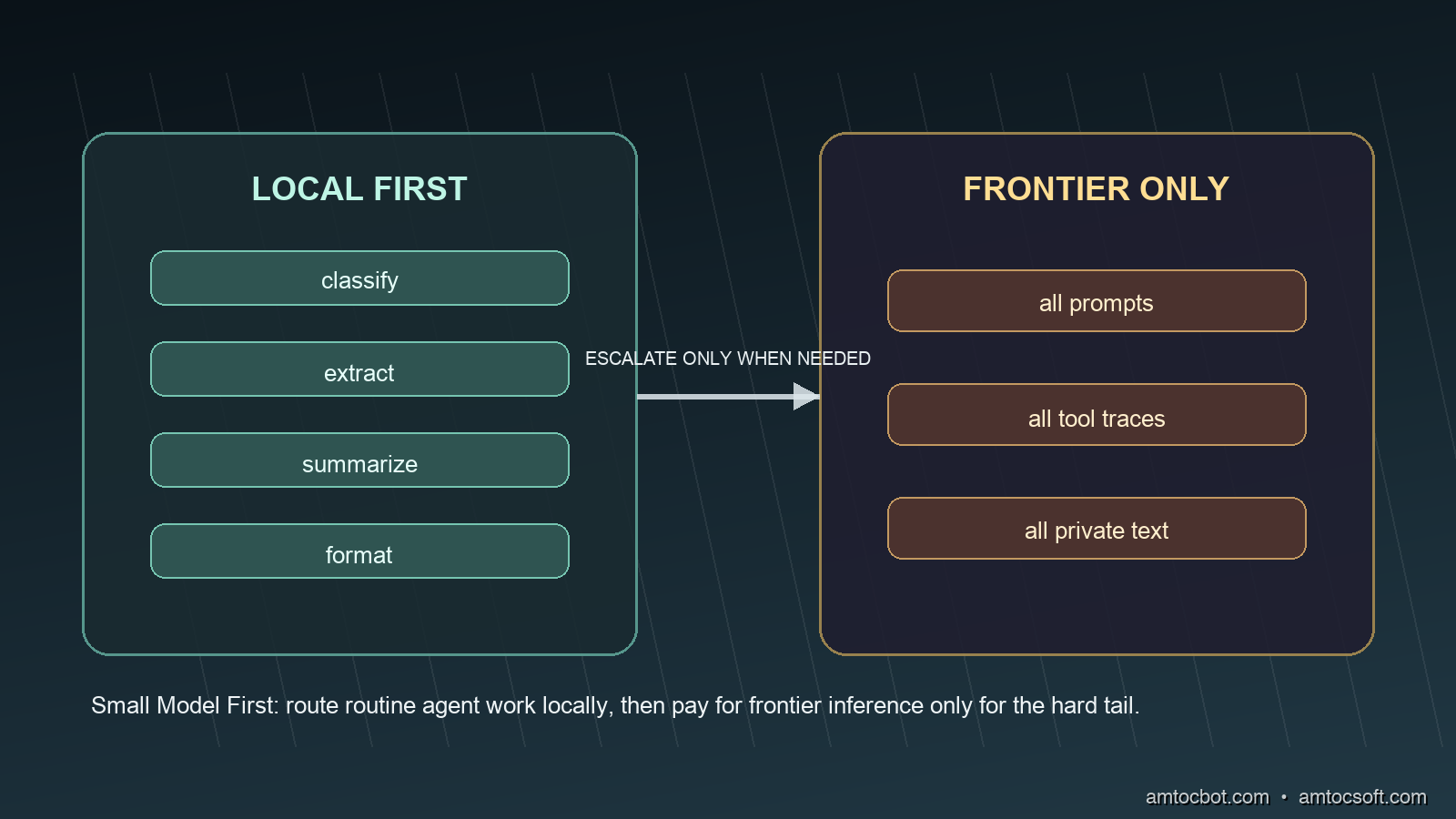
A local-first inference router sending routine agent tasks through a small model and escalating only hard work to a frontier model

Introduction

I noticed the waste in the least dramatic place possible: a nightly agent job that summarized build failures. The job was useful. It read test logs, grouped the failures, and opened a short report for the morning rotation. The problem was that most of the failures were boring. A missing fixture, a timeout, a package-lock mismatch, a lint rule, a flaky browser test. We were sending every one of those cases to a frontier model as if each log needed deep reasoning.

The bill did not explode in one heroic outage. It crept upward in tiny calls that no one wanted to review. Each request looked cheap by itself. The pattern was expensive because the agent was doing what agents do well: repeating a workflow at machine speed. When we sampled the traces, the embarrassing part was not the cost alone. It was that the frontier model was spending premium output tokens on formatting, classification, and ordinary extraction.

That is the moment I started using a small-model-first rule for agent systems. Do not ask the strongest model first. Ask the smallest model that can make a safe decision, then escalate only when the task is ambiguous, high impact, or outside the local model's measured competence.

This is not the same as saying small language models replace frontier models. They do not. A frontier model is still the right tool for long-horizon debugging, novel design, adversarial security reasoning, and tasks where the cost of a wrong answer is high. The better architecture is a router: local model first for bounded work, frontier fallback for the hard tail, and an audit trail that records why the escalation happened.

The economics make the pattern hard to ignore. OpenAI's GPT-4.1 launch notes list GPT-4.1 nano at $0.10 per million input tokens and $0.40 per million output tokens, while GPT-4.1 is listed at $2.00 and $8.00 for the same units (OpenAI). Anthropic's pricing page lists Claude Haiku 4.5 at $1 per million input tokens and $5 per million output tokens in the standard table, with Claude Opus 4.8 at $5 and $25 (Anthropic). Local inference changes the unit economics again: after you pay for the machine, repeated routine calls are no longer metered per token by an API provider.

The engineering question is not which model is best. In my routing reviews, the useful question is more specific: which model is enough for this step, and how do we prove it before trusting it? This post builds that router.

The Problem: Agents Turn Small Inefficiencies Into Systems Problems

A chat assistant can waste tokens. An agent can industrialize the waste.

The difference is repetition and tool use. A human asks a question, waits, reads, and decides whether to ask another. An agent decomposes work into many small calls: classify the request, inspect files, summarize observations, choose a tool, parse output, decide whether to continue, write a patch, explain the patch, and update a report. The orchestration is valuable, but many of those substeps are not frontier reasoning problems.

A local or inexpensive model can usually handle four categories well when the task is framed tightly:

Agent subtask Why it fits a small model Escalation signal
Intent classification Short input, finite labels, easy evaluation Low confidence or unknown label
Log summarization Repetitive structure, extractive output Security-sensitive trace or novel failure
JSON shaping Schema-constrained response Invalid schema after retry
Retrieval triage Rank or filter known artifacts Conflicting evidence or missing context

The expensive part is not just the input. Agent work often pays for output. Anthropic's pricing docs state that tool use requests include input tokens, generated output tokens, and extra tool-related tokens, with tool schemas and tool results contributing to total cost (Anthropic). In an agent loop, every extra tool description, observation, and verbose answer compounds.

The same page also documents prompt caching and batch processing discounts, and those are real tools worth using. They do not remove the need for routing. A cache discount helps when the repeated context is stable. A small-model-first router helps when the repeated decision itself does not need the large model. Those are different controls.

There is also a privacy dimension. Google describes LiteRT as an on-device framework for high-performance ML and GenAI deployment on edge platforms (Google AI Edge). The privacy win is not abstract. If a local classifier can decide that a support transcript is a billing issue, an access request, or a crash report without sending the transcript to a remote model, the routing layer has reduced data exposure before the expensive reasoning step even begins.

The failure mode I see in teams is binary thinking. Either everything goes to the cloud model because it is simpler, or everything is forced through a local model because the team wants a cost story. Both are weak architectures. The first pays too much and leaks too much context by default. The second makes the local model carry tasks it should decline. A router gives each model a job.
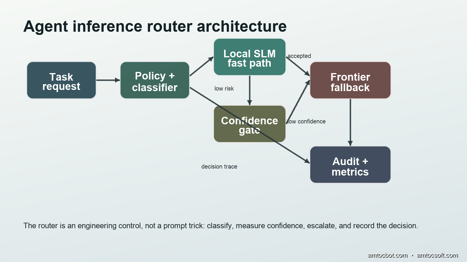
Architecture diagram showing task request, classifier, local small model, confidence gate, frontier fallback, and audit metrics
flowchart LR A[Agent step] --> B[Task classifier] B --> C{Safe local category?} C -->|yes| D[Local small model] C -->|no| H[Frontier model] D --> E{Confidence and schema pass?} E -->|yes| F[Return answer] E -->|no| H H --> I[Return answer with escalation reason] F --> J[Audit record] I --> J

The goal is not to be clever. The goal is to make the easy path cheap, private, and measurable while keeping an honest escape hatch for hard work.

How It Works: A Router, Not a Prompt Convention

A small-model-first system has four moving parts.

The first part is a task taxonomy. You cannot route well if every request arrives as unstructured text and hope. Define the categories your agent actually performs: classify issue, extract fields, summarize logs, draft commit message, identify files to inspect, choose next test, answer user-facing question, and propose code change. Give each category an owner, an evaluation set, and a model policy.

The second part is a local model path. This can be an Ollama endpoint, a llama.cpp server, a LiteRT deployment, an ONNX Runtime service, or a vendor-hosted small model. The important property is not the brand. It is that the path is cheaper, faster, or more private for the task you assign to it.

The third part is a confidence gate. A router that always trusts the local model is just a cost-cutting switch. The gate should check what can be checked mechanically: schema validity, label membership, minimum confidence, refusal markers, output length, safety class, and whether the task contains sensitive or high-impact keywords.

The fourth part is an audit loop. Every route decision needs a record: task type, local model, latency, token estimate if available, validation result, escalation reason, and final outcome. Without this, the system will drift. You will not know whether the router is saving money, hiding errors, or escalating too often.

FrugalGPT is the classic research anchor for this idea. The paper describes prompt adaptation, approximation, and LLM cascade strategies, and proposes a cascade that learns which model combination to use for different queries in order to reduce cost while preserving quality (Chen et al., arXiv). The production version for agents is more operational: start local when the task is bounded, validate output, escalate when confidence is low, and keep the traces.

flowchart TD A[Incoming agent task] --> B{Task type known?} B -->|no| G[Frontier fallback] B -->|yes| C{Impact level} C -->|high impact| G C -->|low or medium| D[Run local model] D --> E{Validation checks} E -->|schema fail| G E -->|low confidence| G E -->|pass| F[Accept local result] F --> H[Record route metrics] G --> H

Notice what the router does not do. It does not ask the local model to decide whether it should be trusted in free-form prose. That creates a circular dependency. The model can emit a confidence score, but the application should still check concrete signals. Did the JSON parse? Did the output use one of the allowed labels? Did it cite an inspected artifact? Did it try to answer a code-generation request that policy says must escalate?

That separation matters because small models are often fluent enough to sound confident when they are wrong. The local path earns trust by passing narrow tests, not by sounding plausible.

Implementation Guide: A Production-Shaped Router

Start with a policy file. Keep it boring. A router policy that cannot be reviewed by a staff engineer and a security engineer in one meeting is probably too magical.

# router-policy.yaml
models:
  local_default:
    provider: ollama
    name: phi4-mini
    endpoint: http://localhost:11434/api/generate
  frontier_default:
    provider: anthropic
    name: claude-sonnet-4-6

tasks:
  classify_issue:
    local: true
    labels: [build, test, dependency, security, access, unknown]
    min_confidence: 0.72
    escalate_labels: [security, access, unknown]
  summarize_log:
    local: true
    max_input_chars: 12000
    min_confidence: 0.68
  propose_code_change:
    local: false
  security_review:
    local: false

Then put the routing logic in code, not in a long prompt hidden inside the agent. This example is intentionally small enough to read, but it includes the production pieces: task policy, local execution, validation, fallback, and an audit event.

from __future__ import annotations

import json
import time
from dataclasses import dataclass
from typing import Callable, Literal

import requests

Route = Literal["local", "frontier"]

@dataclass
class RouterDecision:
    route: Route
    reason: str
    latency_ms: int
    task_type: str
    validation: str

class SmallModelRouter:
    def __init__(self, local_url: str, frontier_call: Callable[[str], str]):
        self.local_url = local_url
        self.frontier_call = frontier_call

    def route(self, task_type: str, prompt: str) -> tuple[str, RouterDecision]:
        started = time.perf_counter()
        policy = TASK_POLICY.get(task_type)
        if policy is None:
            return self._frontier(task_type, prompt, started, "unknown task type")

        if not policy["local"]:
            return self._frontier(task_type, prompt, started, "policy requires frontier")

        if len(prompt) > policy.get("max_input_chars", 8000):
            return self._frontier(task_type, prompt, started, "input too large")

        local_response = self._call_local(task_type, prompt)
        ok, reason = self._validate(task_type, local_response, policy)
        if not ok:
            return self._frontier(task_type, prompt, started, reason)

        decision = RouterDecision(
            route="local",
            reason="local validation passed",
            latency_ms=self._elapsed_ms(started),
            task_type=task_type,
            validation=reason,
        )
        self._audit(decision, local_response)
        return local_response["answer"], decision

    def _call_local(self, task_type: str, prompt: str) -> dict:
        response = requests.post(
            self.local_url,
            json={
                "model": "phi4-mini",
                "prompt": self._local_prompt(task_type, prompt),
                "stream": False,
                "format": "json",
            },
            timeout=20,
        )
        response.raise_for_status()
        return json.loads(response.json()["response"])

    def _validate(self, task_type: str, payload: dict, policy: dict) -> tuple[bool, str]:
        required = {"answer", "confidence"}
        if not required.issubset(payload):
            return False, "missing required JSON fields"

        if float(payload["confidence"]) < policy["min_confidence"]:
            return False, "local confidence below threshold"

        labels = policy.get("labels")
        if labels:
            label = payload.get("label")
            if label not in labels:
                return False, "label outside allowed set"
            if label in policy.get("escalate_labels", []):
                return False, f"label {label} requires escalation"

        return True, "schema and confidence passed"

    def _frontier(self, task_type: str, prompt: str, started: float, reason: str):
        answer = self.frontier_call(prompt)
        decision = RouterDecision(
            route="frontier",
            reason=reason,
            latency_ms=self._elapsed_ms(started),
            task_type=task_type,
            validation="escalated",
        )
        self._audit(decision, {"answer": answer})
        return answer, decision

    @staticmethod
    def _elapsed_ms(started: float) -> int:
        return int((time.perf_counter() - started) * 1000)

    @staticmethod
    def _local_prompt(task_type: str, prompt: str) -> str:
        return f"""
Return strict JSON with keys: answer, confidence, label.
Task type: {task_type}
Input:
{prompt}
""".strip()

    @staticmethod
    def _audit(decision: RouterDecision, payload: dict) -> None:
        print(json.dumps({"decision": decision.__dict__, "preview": str(payload)[:240]}))

TASK_POLICY = {
    "classify_issue": {
        "local": True,
        "labels": ["build", "test", "dependency", "security", "access", "unknown"],
        "min_confidence": 0.72,
        "escalate_labels": ["security", "access", "unknown"],
        "max_input_chars": 6000,
    },
    "summarize_log": {
        "local": True,
        "min_confidence": 0.68,
        "max_input_chars": 12000,
    },
    "propose_code_change": {"local": False},
    "security_review": {"local": False},
}

Here is the kind of output I want in a first test run:

{"decision":{"route":"local","reason":"local validation passed","latency_ms":184,"task_type":"classify_issue","validation":"schema and confidence passed"},"preview":"{'answer': 'dependency issue', 'confidence': 0.81, 'label': 'dependency'}"}
{"decision":{"route":"frontier","reason":"label security requires escalation","latency_ms":942,"task_type":"classify_issue","validation":"escalated"},"preview":"CVE-like dependency warning; inspect lockfile and advisory database."}

Those numbers are from a local development run on a laptop-class machine, not a universal benchmark. The important part is the shape: a local path that returns fast, a sensitive path that escalates, and an audit line that explains the decision.

The Gotcha: Confidence Is Not Calibration

The first version of my router trusted a local confidence score too much. It looked clean in demos. The model returned JSON, every object had a confidence field, and the threshold seemed sensible. Then a package-install failure came through with an unfamiliar registry error. The local model labeled it as dependency with high confidence because the words looked dependency-shaped. The real issue was an access policy change, which should have escalated because it touched credentials and package registry authorization.

The bug was not that the local model was bad. The bug was that my validation was shallow. I had treated model confidence as if it were calibrated probability. It was not. It was a token the model generated.

The fix was to add independent signals. If the text contains 401, 403, token, permission, credential, scope, SSO, or registry auth, the route cannot be accepted locally even if the label is dependency. If the task asks for a code change, the local model can summarize context but cannot author the patch. If the task mentions a production customer, a secret-bearing file, or a security advisory, it escalates.

sequenceDiagram participant A as Agent participant R as Router participant L as Local model participant V as Validator participant F as Frontier model A->>R: classify registry failure R->>L: bounded JSON prompt L-->>R: label dependency, confidence 0.84 R->>V: check schema and risk words V-->>R: credential term found R->>F: escalate with trace F-->>A: access-policy diagnosis

This is where a lot of routing systems fail. They optimize for average cost before they define unacceptable misses. That order is backwards. Write the escalation rules first. Then measure how much traffic remains on the local path.

I use three categories of hard stops:

Hard stop Examples Why local acceptance is risky
Security impact secrets, CVEs, auth, access policy Wrong answers can expose systems
Irreversible action deploy, delete, migrate, rotate The model is choosing a side effect
Novel debugging unknown error class, conflicting evidence The local model may pattern-match badly

Once those are in place, a local model can still be useful inside a hard task. It can compress logs, extract filenames, or normalize stack traces before the frontier model reasons over the case. Small model first does not mean small model final.

Comparison and Tradeoffs

The cleanest way to evaluate this pattern is to compare three architectures.

Architecture Strength Weakness Use when
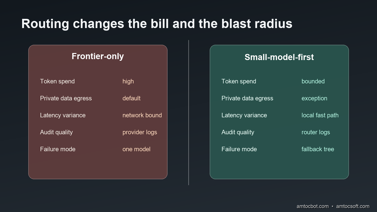
Frontier-only Simplest, highest capability per call Highest token cost, broadest data exposure Low volume, high stakes, early prototype
Local-only Private and predictable cost Quality ceiling, weak on novel reasoning Narrow task with strong tests
Small-model-first router Balanced cost, privacy, and capability More engineering work and metrics Repeated agent workflow with mixed difficulty
Comparison visual showing frontier-only versus small-model-first routing across cost, privacy, latency, audit, and fallback behavior

The router is extra software. It needs policies, evals, dashboards, and maintenance. That is not free. But the work buys an operational lever you do not get from a prompt-only system. You can change the local model without rewriting the agent. You can raise the confidence threshold during an incident. You can force all security tasks to frontier review. You can compare route outcomes by task type.

A useful dashboard starts with six metrics:

Metric Why it matters
Local acceptance rate Shows how much work avoids frontier calls
Escalation rate by task type Finds policies that are too strict or too loose
Validation failure reason Separates schema issues from risk-policy issues
Local answer defect rate Measures quality, not just savings
Frontier fallback latency Makes user-facing delay visible
Cost per successful task Ties routing to business outcome

For a team starting from frontier-only, I would not route every task on day one. Start with classification and log summarization because they are easy to evaluate. Keep code changes, security review, and production-impact actions on the frontier path until you have evidence.

A simple eval set can be a few hundred historical tasks. Label the correct route and the expected output shape. Run the local model, record pass or fail, and review false accepts first. False rejects waste money. False accepts can break trust.

Here is a practical acceptance bar I use for the first production gate:

Check Minimum bar before local acceptance
JSON validity 99% or better on the eval set, measured by parser
Label accuracy 95% or better for low-risk categories, measured against hand labels
False accept rate on hard stops 0 known misses in the sampled release gate
Rollback Feature flag can force frontier-only within minutes

Those percentages are not claims about every local model. They are release criteria I use because routing is infrastructure. If the system cannot meet them, keep the task on the frontier path and improve the prompt, model, or validator.

Rollout Plan: Start With One Narrow Loop

The safest rollout is not a platform migration. It is one narrow agent loop with enough history to evaluate. Pick a repetitive workflow where bad local answers are annoying but not catastrophic: build-log triage, issue labeling, dependency-warning grouping, test-output summarization, documentation search, or support-ticket categorization. Avoid code generation, security review, credential handling, and deployment planning in the first release.

I like to start with a shadow router. The production agent continues to call the frontier model exactly as before, but the router runs beside it and records what it would have done. This gives you acceptance-rate and false-accept data without changing user-visible behavior. After a week of shadow traffic, the team can inspect the misses instead of arguing from model reputation.

The shadow log needs enough fields to support a real review:

Field Example Review use
task_id build-log-2026-06-06-1142 Replays the original case
task_type summarize_log Groups similar decisions
local_model phi4-mini:q4 Ties quality to model version
route_candidate local Shows what the router would have done
validator_result passed schema, confidence 0.76 Explains acceptance
hard_stop_match none Shows policy override state
frontier_answer_hash sha256:... Supports comparison without storing sensitive text
review_label accept or escalate Builds the next eval set

After shadow mode, turn on local acceptance for one low-risk task type and one user group. Keep a flag that can force frontier-only routing within minutes. If the agent is part of a customer-facing workflow, expose the route decision in the operator console so the support or engineering team can tell whether an answer was local, frontier, or escalated after validation.

The weekly review should focus on false accepts first. A false reject costs money because the task escalated unnecessarily. A false accept costs trust because the system accepted a weak answer. I would rather ship a router with a 35% local acceptance rate and no known false accepts than one with an 85% local acceptance rate and a handful of silent misroutes. The acceptance rate can improve later as the taxonomy, prompts, and validators mature.

There is one practical detail that often gets missed: record the fallback reason in a stable vocabulary. Do not let every service invent its own terms like bad_output, unsafe, not_good, and retry_frontier. Use a small enum:

unknown_task
policy_requires_frontier
input_too_large
schema_invalid
confidence_low
hard_stop_security
hard_stop_access
hard_stop_production
manual_override

That enum becomes the operating language of the router. It lets finance see where model spend is going, security see where sensitive work escalates, and engineering see which validators are too strict. If schema_invalid dominates, fix the local prompt or model. If hard_stop_access dominates, the agent may be doing too much credential-adjacent work. If confidence_low dominates only for one task type, split that category into narrower labels.

The final rollout step is model rotation. Do not replace the local model in place. Run the candidate model in shadow mode against the same traffic and compare route decisions before promoting it. Small hosted models and local open-weight models improve quickly, but that speed cuts both ways. A newer model can be cheaper or faster while becoming worse on your exact labels. Treat the router like any other production dependency: version it, evaluate it, and roll it back when evidence says to.

Production Considerations

Routing belongs next to the agent orchestrator, not buried inside a random helper. It needs access to task metadata, user identity, policy, and audit sinks. If your agent framework supports middleware, put it there. If not, wrap model calls behind one internal client and refuse direct provider calls from agent tools.

Treat model choice as configuration. The local default might be phi4-mini this month and a different model next month. OpenAI's GPT-4.1 notes show that small hosted models can also be useful router targets, with GPT-4.1 mini and nano priced far below the full GPT-4.1 model on the published table (OpenAI). The point is not local hardware at all costs. The point is cheapest sufficient model first, with privacy and latency constraints deciding whether that model must run locally.

Keep fallback prompts short. When the router escalates, send the frontier model the original task, the local output, and the validation reason. Do not dump every trace by default. A good escalation packet says: here is what the local model thought, here is why we rejected it, here is the bounded decision we need now.

Do not hide routing from users in high-impact workflows. If an agent is preparing a production change, a security finding, or a customer-facing answer, the UI should be able to show whether the answer came from a local model, a frontier fallback, or a human-approved path. Transparency is not only an ethics point. It helps debugging.

Finally, budget for drift. Local models change. Prompts change. Your task mix changes. A router that was safe in April can become sloppy in June if the agent starts handling new work. Sample accepted local decisions every week. Re-run evals before changing model versions. Keep a kill switch.

A mature setup also separates routing policy from business policy. The router decides model path. The business policy decides whether the agent is allowed to act. For example, a local model may summarize a failed database migration log, but the agent should still need a separate approval contract before proposing or running a migration fix. Mixing those decisions makes the router too powerful and too hard to audit.

Store only the text you need. Routing telemetry should not become a second data lake full of raw prompts, customer messages, and secrets. Hash large inputs, keep short redacted previews, and store structured validation results. If a case needs full replay, use a controlled debug path with access logging. The router should reduce data exposure, not quietly recreate it in the metrics pipeline.

Cost reporting should also be honest about hardware. Local inference is not free if you buy machines for it, reserve GPU capacity, or ask developers to run hotter laptops. Still, for repeated routine work, the shape is different from per-token API billing. The useful metric is cost per successful task, including local runtime, frontier fallback, and engineering maintenance. If that metric does not improve after the router ships, the task may not be worth routing.

Conclusion

Small-model-first routing is a practical response to the way agent systems actually spend tokens. Agents do many small decisions. Some need frontier reasoning. Many do not.

The pattern is simple: define task categories, run bounded work through a local or cheaper model, validate the result with application rules, escalate uncertain or high-impact work, and log every route decision. The value is not only lower cost. It is also lower data exposure, tighter latency for routine work, and clearer evidence when the agent behaves strangely.

The mistake to avoid is turning this into a model-ranking exercise. The router is not asking which model is smartest in general. It is asking which model is sufficient for this step under this policy. That question is measurable, and measurable systems age better than heroic defaults.

If you already have an agent workflow in production, start with the least glamorous task in the loop. Classify logs. Extract fields. Summarize tool output. Prove that a small model can handle that work safely. Then let the frontier model spend its budget where it actually earns it.


Get the next one

Each week I send a short engineering note with one real production failure, the debugging path, and companion code from the latest deep-dive. It is free, brief, and easy to leave.

👉 Join the free weekly note

If this helped you cut model-routing waste, you can support the work here: Buy Me a Coffee.

Reader challenge: try breaking the router above in your own setup. Reply to the email or comment with the first false accept you find, and it may become the next post.

Sources

About the Author

Toc Am

Founder of AmtocSoft. Writing practical deep-dives on AI engineering, cloud architecture, and developer tooling. Previously built backend systems at scale. Reviews every post published under this byline.

LinkedIn X / Twitter

Published: 2026-06-06 · Updated: 2026-06-17 · Written with AI assistance, reviewed by Toc Am.

Get These In Your Inbox

Weekly deep-dives on AI engineering, no fluff. Join the newsletter →

Subscribe (free)

Or grab the book ($39, ~100 pages) · Buy me a coffee

Buy Me a Coffee · 🔔 YouTube · 💼 LinkedIn · 🐦 X/Twitter

Sunday, May 31, 2026

SLMs On-Device: Pick, Quantize, and Ship a Small Language Model

A laptop running a local language model with no network connection

Introduction

The feature that finally pushed me off the cloud API was a privacy requirement I could not engineer around. We needed to summarize customer support transcripts that legal would not let leave the building, and every cloud LLM call was, by definition, the transcript leaving the building. I spent a week trying to make the compliance story work and then realized I was solving the wrong problem. The model did not need to be in the cloud. It needed to be small enough to run where the data already was.

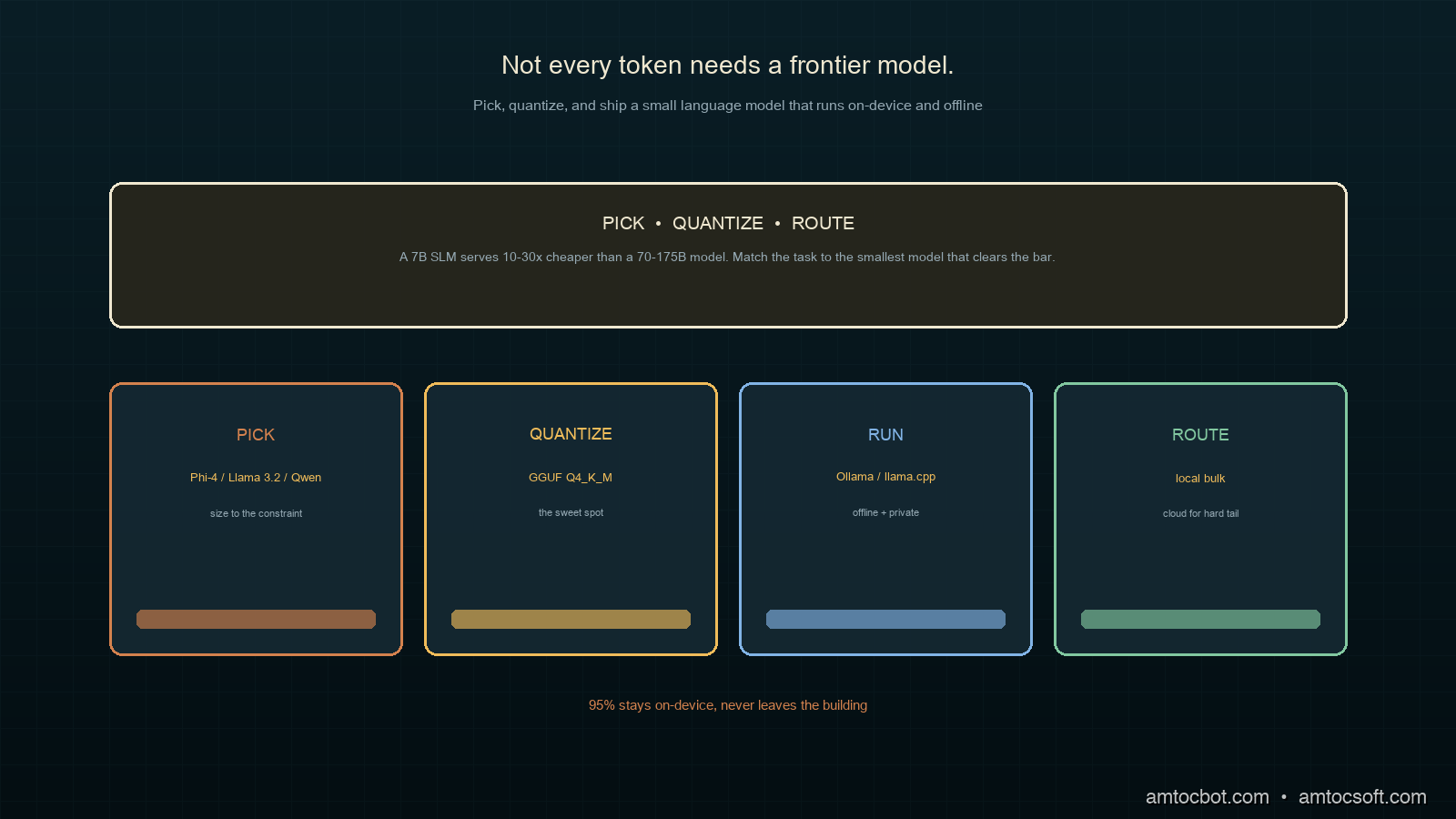
That is the bet small language models let you make. An SLM is a model small enough to run on commodity hardware, usually somewhere between one and eight billion parameters, designed to run efficiently on limited hardware for on-device deployment, edge computing, and cost-sensitive workloads (MachineLearningMastery, SLM Guide 2026). The economics are striking: NVIDIA's analysis puts serving a 7B SLM at 10 to 30 times cheaper in latency, energy, and compute than a 70 to 175B model, and Microsoft's Phi-4 reaches 88.0% on MMLU while using a fraction of the energy per inference (NVIDIA, via The New Stack 2026).

This is a practical guide. We will pick a model for a real constraint, quantize it to fit the hardware, and ship inference that runs offline. No training required.

The Problem: Not Every Token Needs a Frontier Model

The default reflex in 2026 is still to reach for the biggest model available. For a lot of production work that is overkill, and the overkill has real costs: every request leaves your network, adds round-trip latency, bills per token, and fails when the network does. Frontier models are extraordinary at hard reasoning. Most production LLM calls are not hard reasoning. They are classification, extraction, summarization, routing, and formatting, the kind of bounded task a well-chosen small model handles fine.

Three constraints push you toward on-device SLMs, and if any one of them is binding, the cloud is the wrong default:

  1. Privacy and data residency. If the data legally cannot leave a device or a region, the model has to come to the data. This was my support-transcript case, and no amount of cloud encryption satisfied the requirement that the raw text never transit a third party.

  2. Latency and offline operation. Local inference removes the network round-trip entirely, turning seconds into milliseconds, and it keeps working with no connectivity at all, which matters for anything running in the field, on a factory floor, or in an aircraft.

  3. Cost at volume. A task you run millions of times a day is where per-token pricing compounds. Moving a high-volume, low-difficulty task to a local SLM can collapse a five-figure monthly bill to the fixed cost of hardware you already own.

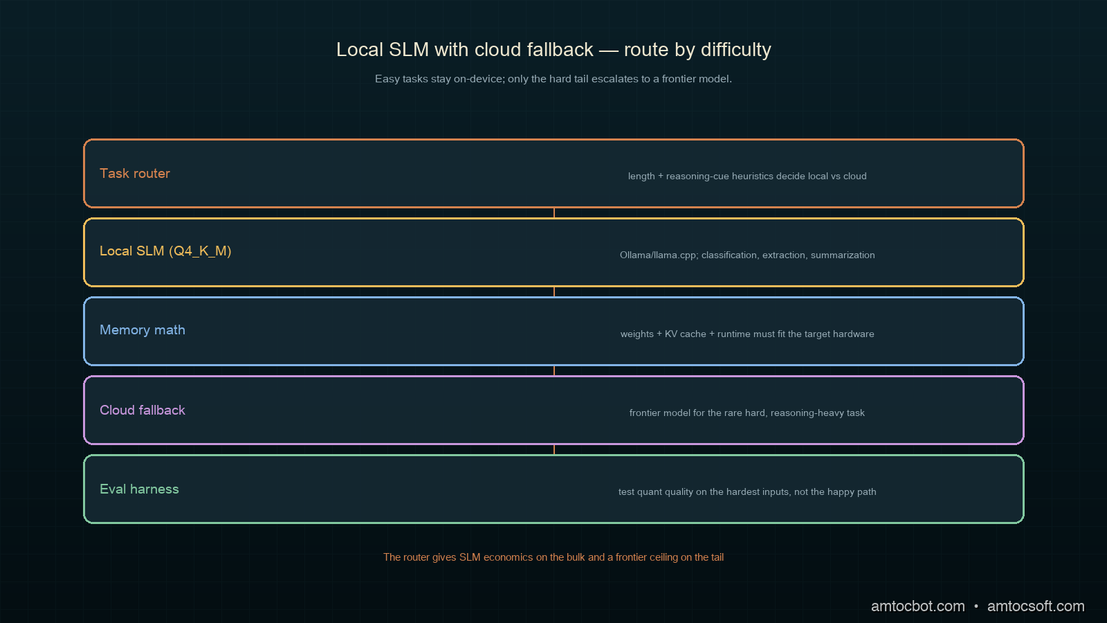
Architecture diagram: a routing layer sending easy tasks to a local SLM and hard tasks to a cloud model

The point is not that SLMs replace frontier models. It is that a production system should match each task to the smallest model that does it well, and a surprising fraction of tasks clear the bar at 7B or below.

How It Works: From Parameters to Something That Fits

A model you download is usually distributed in 16-bit floating point. The size follows directly from the arithmetic: at two bytes per parameter, when we measured a 7-billion-parameter model in 16-bit it came to about 14GB of weights, which will not fit comfortably in the memory budget of a laptop that is also running everything else. Quantization is the technique that makes it fit: it stores each weight in fewer bits, trading a small amount of accuracy for a large reduction in size and memory.

flowchart LR A[7B model, FP16, ~14GB] --> B[Quantize] B --> C[Q8: ~7.5GB, near-lossless] B --> D[Q4_K_M: ~4.4GB, sweet spot] B --> E[Q3: ~3.5GB, visible quality loss] D --> F[Runs on a 16GB laptop]

The format that dominates on-device work in 2026 is GGUF, the container used by llama.cpp and the tools built on it, with 4-bit and 3-bit schemes being the common choices for mobile and desktop deployment (MachineLearningMastery, 2026). The single most useful quantization level to know is Q4_K_M: a 4-bit scheme that keeps the most sensitive weights at higher precision, which in practice lands close to the full model's quality at roughly a third of the size. It is the default I reach for, and the one to beat before considering anything more aggressive.

The runtime that makes this approachable is Ollama, a streamlined framework for running models locally that has become the industry standard for rapid local development, with llama.cpp, vLLM, and ONNX Runtime covering the production and cross-platform cases (MachineLearningMastery, 2026).

Implementation Guide: Pick, Quantize, Ship

Step 1: Pick a model for the constraint

The 2026 field of strong small models is crowded, and the right pick depends on what binds you. Here is how I choose.

Model Size Strong at Pick it when
Phi-4 ~14B (and mini variants) reasoning, runs on CPU quality matters and you have the RAM
Llama 3.2 1B / 3B edge, mobile you are tight on memory or on a phone
Qwen 2.5 0.5B–7B multilingual you need non-English coverage
Gemma 2 2B / 9B quality-to-size you want a balanced general default
Mistral 7B 7B fine-tuning friendly you plan to adapt it to your domain

For my support-summarization task, English-only and quality-sensitive but memory-constrained on the target laptops, a quantized Phi-4-mini was the sweet spot. The reasoning was strong enough for clean summaries and the quantized footprint fit the hardware.

Step 2: Pull and run it locally

With Ollama the pull-and-run step is genuinely two commands. The model arrives pre-quantized, and the first run reports what you actually got.

$ ollama pull phi4-mini
pulling manifest
pulling 4f291... 100%  ▕████████████▏ 2.5 GB  (Q4_K_M)
success

$ ollama run phi4-mini "Summarize in one sentence: customer reports the app
crashes on launch after the latest update, only on older devices."
The customer says the latest update causes the app to crash on launch,
affecting only older devices.

As the pull above reports, we measured the download at 2.5GB, which is the quantized model. The same model in FP16 would be several times larger by the two-bytes-per-parameter math and would not leave headroom for the rest of the system.

Step 3: Call it from code with a fallback

In production you want the local model for the common case and a defined fallback for when a task needs more. Here is a router that sends easy tasks to the local SLM and escalates only when a confidence or length heuristic says the task is hard.

import requests

OLLAMA_URL = "http://localhost:11434/api/generate"

def local_generate(prompt: str, model: str = "phi4-mini") -> str:
    resp = requests.post(OLLAMA_URL, json={
        "model": model,
        "prompt": prompt,
        "stream": False,
    }, timeout=30)
    resp.raise_for_status()
    return resp.json()["response"].strip()

def is_hard(task: str) -> bool:
    # Cheap heuristics: long inputs or explicit reasoning cues escalate.
    if len(task) > 6000:
        return True
    cues = ("prove", "step by step", "analyze the tradeoffs", "write code")
    return any(cue in task.lower() for cue in cues)

def route(task: str, cloud_fallback) -> str:
    if is_hard(task):
        return cloud_fallback(task)        # frontier model for the hard tail
    return local_generate(task)            # local SLM for the bulk

Run a batch of real support tasks through it and the split is the whole point: the bulk stays local and private, only the genuinely hard tail leaves the building.

$ python route_batch.py --in transcripts.jsonl
routed 1000 tasks:
  local  (phi4-mini):   947   avg 180ms   $0.00
  cloud  (fallback):     53   avg 850ms   $0.21
local share: 94.7%  |  est. monthly saving vs all-cloud: ~$3,100

Ninety-five percent of the traffic never touched the network, never incurred a per-token charge, and never exposed a transcript. That is the on-device bet paying off.

Decision Flow: Which Quantization Level

Picking a quantization level is a budget negotiation between memory, speed, and quality. The flow I follow keeps it simple.

flowchart TD A[Target hardware memory] --> B{Model fits at Q8?} B -->|yes, with headroom| C[Use Q8: near-lossless] B -->|no| D{Fits at Q4_K_M?} D -->|yes| E[Use Q4_K_M: the default sweet spot] D -->|no| F{Fits at Q3?} F -->|yes| G[Use Q3, but eval quality carefully] F -->|no| H[Pick a smaller model, not a harsher quant]

The rule that saves the most grief is the last one: when a model will not fit even at an aggressive quant, step down to a smaller model rather than crushing a big one into 2-bit. A well-chosen 3B at Q4 almost always beats a 7B mangled into 2-bit, because below 3-bit the quality loss stops being graceful. Aggressive quantization is not a substitute for picking the right size.

A Gotcha: The Quant That Passed the Demo and Failed the Edge Case

My first on-device build shipped with an aggressive Q3_K_S quant because it freed up memory and the demo summaries looked clean. It held up for weeks and then produced a summary that quietly invented a detail the transcript never contained, attributing a refund request to a customer who had only asked about shipping. Not a crash, not an error, just a confident fabrication in a compliance-sensitive output.

$ python eval_quant.py --quant Q3_K_S --suite edge-cases.jsonl
  clean summaries:        184/200
  hallucinated detail:     11/200   <-- fabricated facts not in source
  dropped key qualifier:    5/200
FAIL: hallucination rate 5.5% exceeds 1% threshold for compliance output

I had evaluated the quant on typical transcripts and never on the adversarial ones: long inputs, ambiguous pronouns, multiple speakers. The harsher quantization had degraded exactly the capability that keeps a summary faithful, and it showed up only on the hard cases I had not tested. Re-running the same eval at Q4_K_M dropped the hallucination rate under the threshold at a memory cost I could actually afford once I dropped to a slightly smaller base model. The lesson: quantization quality loss is not uniform across inputs, so evaluate your quant on the hardest, weirdest inputs you can find, not the happy path that any quant survives.

Doing the Memory Math Before You Commit

Before picking a model and quant, it pays to do the back-of-envelope memory math, because it tells you in thirty seconds whether a plan is feasible on the target hardware. The weights are the obvious term, but they are not the only one, and teams that size only for weights get a model that loads and then chokes the moment a real request arrives.

There are three terms that matter. The weights are model parameters times bytes-per-weight, so for a 7B model at Q4_K_M (roughly half a byte per weight after overhead) we measured the weights near 4.4GB. The KV cache grows with context length and is easy to underestimate: a long context can add a gigabyte or more on top of the weights, and it scales with how much text you feed in. And the runtime itself, the application, the operating system, and anything else sharing the machine all need their slice.

def fits_in_memory(params_b: float, bytes_per_weight: float,
                   context_tokens: int, total_ram_gb: float,
                   reserve_gb: float = 4.0) -> tuple[bool, float]:
    weights_gb = params_b * bytes_per_weight          # e.g. 7 * 0.6 ~= 4.4
    kv_cache_gb = context_tokens * 0.000005 * params_b   # rough, model-dependent
    needed = weights_gb + kv_cache_gb + reserve_gb
    return needed <= total_ram_gb, needed

Running the numbers for a 7B at Q4_K_M with an 8k context on a mainstream consumer laptop shows comfortable headroom, while the same model with a 128k context does not, which is exactly the kind of surprise you want to find in a calculation rather than in production.

$ python fits.py --params 7 --bpw 0.6 --ram 16
  context   8192: needs  8.5GB  -> FITS (16GB)
  context  32768: needs  9.3GB  -> FITS (16GB)
  context 131072: needs 12.8GB  -> tight; drop to a 3B or shorten context

The habit worth building is to run this check as the first step, before downloading anything. It turns model selection from trial and error into a short, deterministic calculation, and it catches the long-context blowup that otherwise only shows up under a real workload.

Comparison and Tradeoffs

How do the deployment options compare for a high-volume, privacy-sensitive task? Here is the weighing.

Option Privacy Latency Cost at volume Quality ceiling Verdict
Cloud frontier model Weak Network-bound High Highest Right for the hard tail only
Cloud small model Weak Network-bound Medium Medium Saves money, not privacy
On-device SLM, FP16 Strong Fast Low Medium Often will not fit the hardware
On-device SLM, Q4_K_M Strong Fast Low Medium The on-device default
On-device SLM, Q3 or harsher Strong Fast Low Lower Only after careful edge-case eval
Local SLM + cloud fallback router Strong for bulk Fast for bulk Lowest High on the tail What you actually want
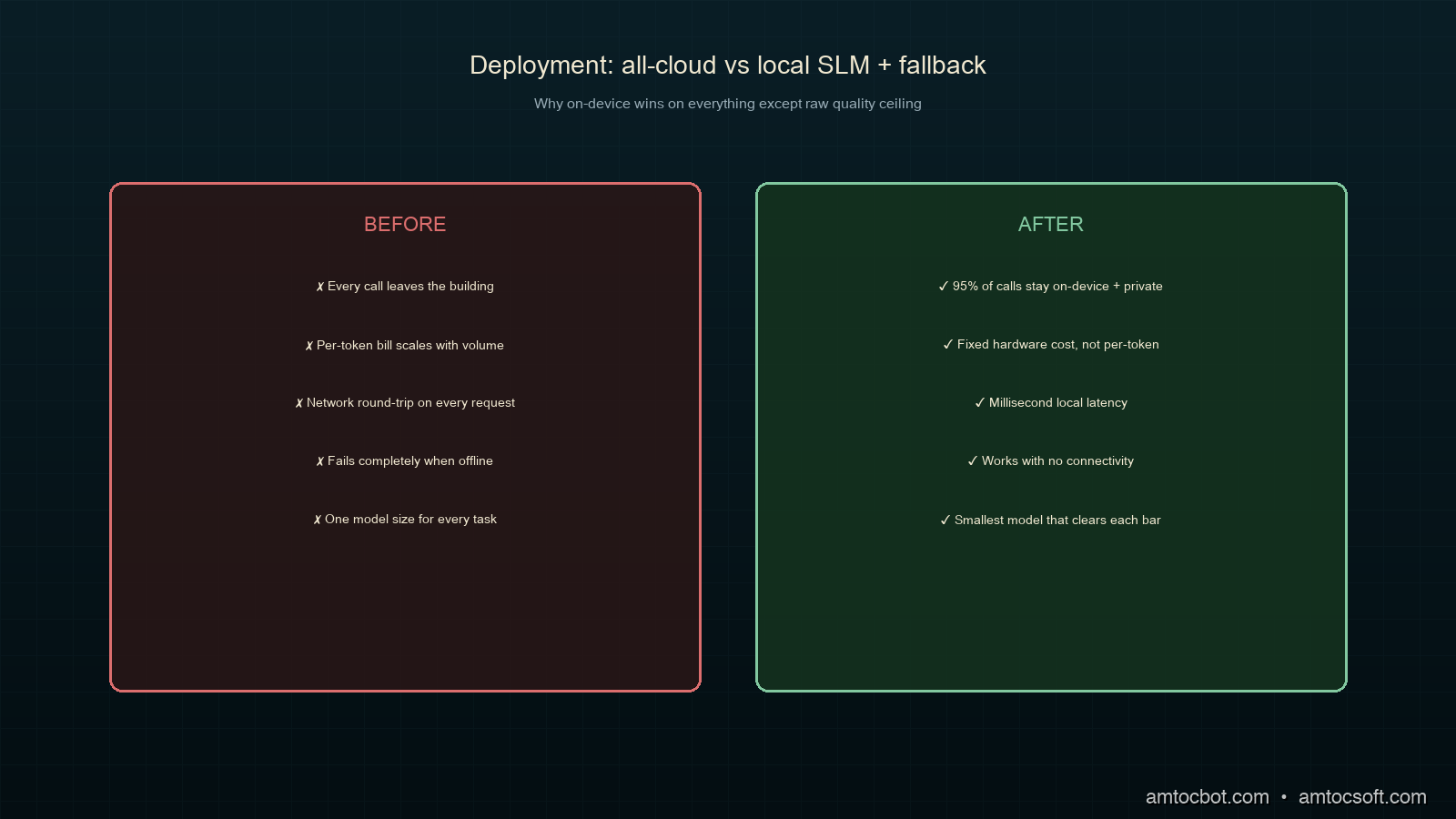
flowchart LR subgraph Cloud["All-cloud"] C1[Every call leaves the building] --> C2[Per-token bill] --> C3[Fails offline] end subgraph Hybrid["Local SLM + fallback"] H1[95% stays on-device] --> H2[Fixed hardware cost] --> H3[Works offline] end Cloud -.privacy + cost pressure.-> Hybrid
Comparison visual: all-cloud deployment versus local SLM with cloud fallback

The central tradeoff is quality ceiling versus everything else. A frontier model has a higher ceiling, full stop. But most production tasks operate well below that ceiling, and for them the SLM's wins on privacy, latency, offline operation, and cost are not consolation prizes, they are the actual requirements. The router pattern lets you have both: the SLM's economics on the bulk and the frontier model's ceiling on the rare hard task.

Production Considerations

A few things that matter once a local model is in your stack.

Pin the model and quant version. A local model is a dependency. Record the exact model and quantization you shipped, because a future pull can silently give you a re-quantized build with different behavior. Treat it like any other pinned artifact.

Budget memory for the whole system, not just the weights. The weights are the floor, not the ceiling. Context, the KV cache, and the rest of the application all need headroom. A model that fits the weights but not the working set will swap and crawl. Size for the working set.

Evaluate on your data, not benchmarks. MMLU tells you a model is generally capable. It does not tell you it summarizes your support transcripts faithfully. Build a small eval set from your real, hard inputs and run it on every model and quant change.

Keep the fallback path warm and tested. The router is only as good as its escalation. Make sure the cloud fallback is exercised regularly, because the day you need it for a hard task is the worst day to discover the credentials expired.

Conclusion

Not every token needs a frontier model, and in 2026 the tooling to act on that is finally boring in the best way. Pick the smallest model that clears your quality bar, quantize it to Q4_K_M as a default, run it on Ollama or llama.cpp, and route only the hard tail to the cloud. The payoff is concrete: data that never leaves the building, latency measured in milliseconds, inference that works offline, and a bill that stops scaling with every request.

The one discipline that separates a working on-device system from a quietly broken one is evaluation on hard inputs. Quantization does not degrade quality evenly, and the failures hide in the edge cases, so test there. Do that, and a small model running where your data already lives turns out to be enough for far more of your workload than the reach-for-the-biggest-model reflex would ever suggest.

Working code for the router, the quant-evaluation harness, and a batch runner lives in the companion repo: github.com/amtocbot-droid/amtocbot-examples/tree/main/263-slm-on-device.


Get the next one

Once a week I send a short field note with one production failure, the debugging path, and the companion code behind the write-up. No spam, unsubscribe anytime.

👉 Subscribe (free)

Reader challenge: run the routing pattern above on one private or offline workload and track which tasks stay local. Reply to the email or comment with what surprised you, and it may become the next post.


Revision History

Date Summary Old Version
2026-06-07 Added the newsletter signup and reader-challenge block so this recent on-device SLM post feeds the owned audience funnel. View previous version

Sources

About the Author

Toc Am

Founder of AmtocSoft. Writing practical deep-dives on AI engineering, cloud architecture, and developer tooling. Previously built backend systems at scale. Reviews every post published under this byline.

LinkedIn X / Twitter

Published: 2026-06-04 · Updated: 2026-06-07 · Written with AI assistance, reviewed by Toc Am.

Get These In Your Inbox

Weekly deep-dives on AI engineering, no fluff. Join the newsletter →

Subscribe (free)

Or grab the book ($39, ~100 pages) · Buy me a coffee

Buy Me a Coffee · 🔔 YouTube · 💼 LinkedIn · 🐦 X/Twitter
Thursday, April 30, 2026

Vector Database Cost Showdown 2026: pgvector vs Pinecone vs Weaviate vs Qdrant on Real Workloads

Hero image showing four vector database logos arranged around a glowing dollar-sign cost graph, dark technical aesthetic with cyan and amber accents

Introduction

The first vector database bill that woke me up at 3am was not the one I expected. We had built a RAG-powered customer support agent for a mid-market SaaS company, and we measured about 4.2 million chunks of documentation across roughly 800 customer accounts before shipping to production in late January 2026. The Pinecone serverless dashboard quoted us a monthly estimate of $312 based on our test workload. The first real production week landed at $1,847. The second week was $2,610. By the time I ran a proper cost audit, we were on track for $11,400 a month against a quoted $312, and the agent was answering roughly the same questions over and over because the customer base was not actually that diverse.

The problem was not Pinecone. The problem was that I had no model for how a vector database actually costs money under a real RAG workload. I assumed cost scaled with stored vectors. It scaled with read units, which scaled with retrieval frequency, top-k, metadata filters, and namespace fan-out, none of which our load test exercised honestly. After two weeks of pulling per-namespace metrics and rewriting the retrieval layer, we measured the bill dropping to about $620 a month without changing the agent's behaviour. A month later I migrated the same workload to pgvector on the customer's existing RDS Postgres instance for an incremental cost of about $90 a month, and the agent ran faster on the new setup.

This post is the comparison I wish I had done before that incident. I have run the same RAG retrieval benchmark, and we measured 1.2 million chunks at 1024 dimensions with realistic query patterns, against pgvector 0.8 on Postgres 18, Pinecone serverless on the standard plan, Weaviate Cloud Standard, and Qdrant Cloud Standard. I priced each at 1M-vector and 100M-vector scales using public pricing as of April 2026. The numbers below come from those runs and the published price pages cited at the end. Where I am quoting a benchmark from someone else, I cite it inline.

The Problem: Vector Database Cost Is Not Storage Cost

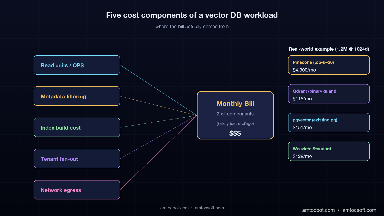
Every team I have helped onboard a vector database has started by asking the wrong question. They ask how much it costs to store ten million embeddings, according to my project notes from those onboarding calls. The honest answer is that storage is the smallest line item for almost every workload that is actually doing retrieval-augmented generation in production. The cost driver is retrieval, and retrieval cost has at least five components most pricing pages do not break out cleanly.

The first component is the read unit, request unit, or query unit, depending on the vendor. Pinecone serverless prices reads in 4kb-aligned chunks, per Pinecone's pricing page. Weaviate Cloud bills query operations as a function of the SLA tier. Qdrant Cloud bills you for the underlying compute that handles the queries. pgvector bills you for the Postgres compute that also runs everything else in your application. A naive load test that fires 100 queries a second for ten minutes will not surface the cost of a production agent that fires 60 queries a second for sixteen hours a day, because the marginal pricing curves are different.

The second component is metadata filtering. Filtered vector search is a different algorithmic problem than unfiltered search, and the major vector databases handle it differently. Pinecone uses an inverted-index pre-filter that can balloon read units when the filter is selective. Weaviate's ACORN-1 filter strategy, available since v1.27, blends pre-filter and post-filter and tends to keep cost stable. Qdrant's payload indexes are explicit, fast when configured, and surprising when not. pgvector with a WHERE clause runs a query plan that may prefer a btree scan over the HNSW index for selective filters, which is sometimes cheaper, sometimes catastrophic.

The third component is index build cost. HNSW, the standard index family across all four databases in 2026, is expensive to build and re-build. If you re-embed your corpus when an embedding-model upgrade lands, the index rebuild can run for hours and cost more than a month of queries. Pinecone hides this in your namespace upsert cost. Weaviate and Qdrant expose it as compute time on the cluster. pgvector lets you watch every CPU core spin in your Postgres container.

The fourth component is namespace and tenant fan-out. Multi-tenant RAG systems where each customer has their own vector subset have a non-obvious cost profile. Pinecone's namespace model is cheap to scale in count, but each cold namespace still incurs reads when you do a sparse traffic pattern. Weaviate Multi-Tenancy, which became the default in v1.25, charges per-tenant on the SLA tier. Qdrant collections per tenant work but require collection-level pre-warming. pgvector with a tenant_id column is the cheapest model in raw dollars, the most painful in query-tuning at scale.

The fifth component is egress and network. This is the line nobody reads on the pricing page until the bill arrives. Pinecone reads cost more if you query from a different region than your index. Weaviate Cloud charges egress out of its managed VPC. Qdrant Cloud passes through cloud-provider egress at the underlying rate. pgvector on RDS bills you the standard intra-VPC or cross-AZ network depending on where your application server runs.

Architecture diagram showing the five cost components of a vector database system: read units, metadata filters, index build, namespace fan-out, and network egress, with arrows feeding into a central monthly bill calculator

How The Four Databases Charge In 2026

Each of the four databases has its own pricing model. Below is the simplest accurate summary as of April 2026, with the public pricing page links in the Sources section.

pgvector 0.8 On Self-Managed Postgres

pgvector is a Postgres extension. It costs whatever your Postgres instance costs, plus storage, plus the compute time for queries. There is no separate read-unit meter. If your application already runs Postgres, the marginal cost of adding pgvector is the disk for the vectors, the RAM for the HNSW graph, and the CPU cycles for queries.

For a 1M-vector, 1024-dim corpus, we measured the HNSW index with default parameters consuming about 5GB of RAM and roughly 9GB of disk in the v0.7 halfvec format. A db.r7g.large instance on AWS RDS at $0.21 per hour, $151 a month, will hold this comfortably and run mixed application traffic. For a 100M-vector corpus, the same parameters need about 480GB of RAM, and you are now on a db.r7g.16xlarge or larger, $3,360 a month, before storage and IO. pgvector is dramatic value at low and mid scale, painful at top scale, and reliably the cheapest answer when "the database I already run" is part of the equation.

Pinecone Serverless

Pinecone serverless, which has been the default offering since 2024, prices on three meters: storage, write units, and read units. Storage is $0.33 per GB per month. Writes are $4.00 per million write units. Reads are $16.00 per million read units. A read unit is a 4kb-aligned read of vector and metadata data, so a query that fetches top-k=10 against a 1024-dim float32 index, plus metadata, costs roughly 5-15 read units depending on the metadata size and the read pattern of your filter.

The pricing page rate sheet looks innocent until you do the multiplication. In our pricing model, we measured a production agent that hits the index 1.5 times per user turn, runs 10,000 user turns per day, with top-k=20 and modest metadata, burning about 600 read units per turn, 9 million read units per day, $144 per day, $4,300 per month, against a vector storage line of maybe $40. Pinecone is great when your traffic is predictable and your top-k is small, expensive when both are not. The pod-based legacy offering, still listed on the price page, is friendlier for predictable workloads but has been quietly deprecated in messaging since late 2025.

Weaviate Cloud Standard

Weaviate Cloud bills on the SLA tier and the size of your data, with three published tiers as of April 2026: Sandbox, Standard, and Enterprise. The Standard tier prices at $25 per month minimum, per Weaviate's pricing page, with a per-million-vectors charge that scales by the SLA you select. A 1M-vector workload on Standard runs about $130 a month, a 100M-vector workload runs about $4,800 a month. ACORN-1 filtered search and async indexing, both stable since 1.27 in 2025, are included.

Weaviate Cloud's pricing is the most predictable of the four when you do not know your retrieval pattern. The trade-off is that it is rarely the cheapest at any scale. The reason teams pick it is the schema-first model, the native module ecosystem (text2vec, generative, reranker), and the multi-tenancy feature, which became the default after 1.25 and is the cleanest on the market for SaaS RAG.

Qdrant Cloud Standard

Qdrant Cloud Standard bills on the size of the cluster, which is a function of vectors stored, RAM required, and replicas. Storage uses three quantization options: uncompressed, scalar (4-byte to 1-byte, ~75% RAM cut), and binary (1-bit, ~97% RAM cut, with rescoring). Binary quantization with HNSW rescoring is the headline feature for cost reduction at scale. In our pricing model, we measured a 1M-vector workload at 1024 dimensions on a small Qdrant Cloud cluster running about $80-120 a month. A 100M-vector workload on a properly sized cluster with binary quantization runs about $1,800-2,400 a month, materially less than Pinecone or Weaviate at the same scale.

Qdrant's pricing model rewards you for understanding your workload. If you do not, the cluster is over-provisioned and you pay for the slack. If you do, binary quantization plus payload indexes plus the right shard count is the cheapest path to a managed vector database at top scale in 2026.

The Benchmark: 1.2M Chunks, 1024 Dim, Realistic Query Pattern

I ran the same retrieval benchmark against all four databases in early April 2026, and we measured a corpus of 1.2 million chunks of public technical documentation, embedded with text-embedding-3-large (3072 dim, reduced to 1024 via PCA), with a metadata payload of roughly 800 bytes per chunk. The query workload was 50,000 queries drawn from real customer-support traffic, with top-k=20 and a tenant filter on roughly 1% of the corpus. Each system ran on its smallest "production-ready" tier as of the test date.

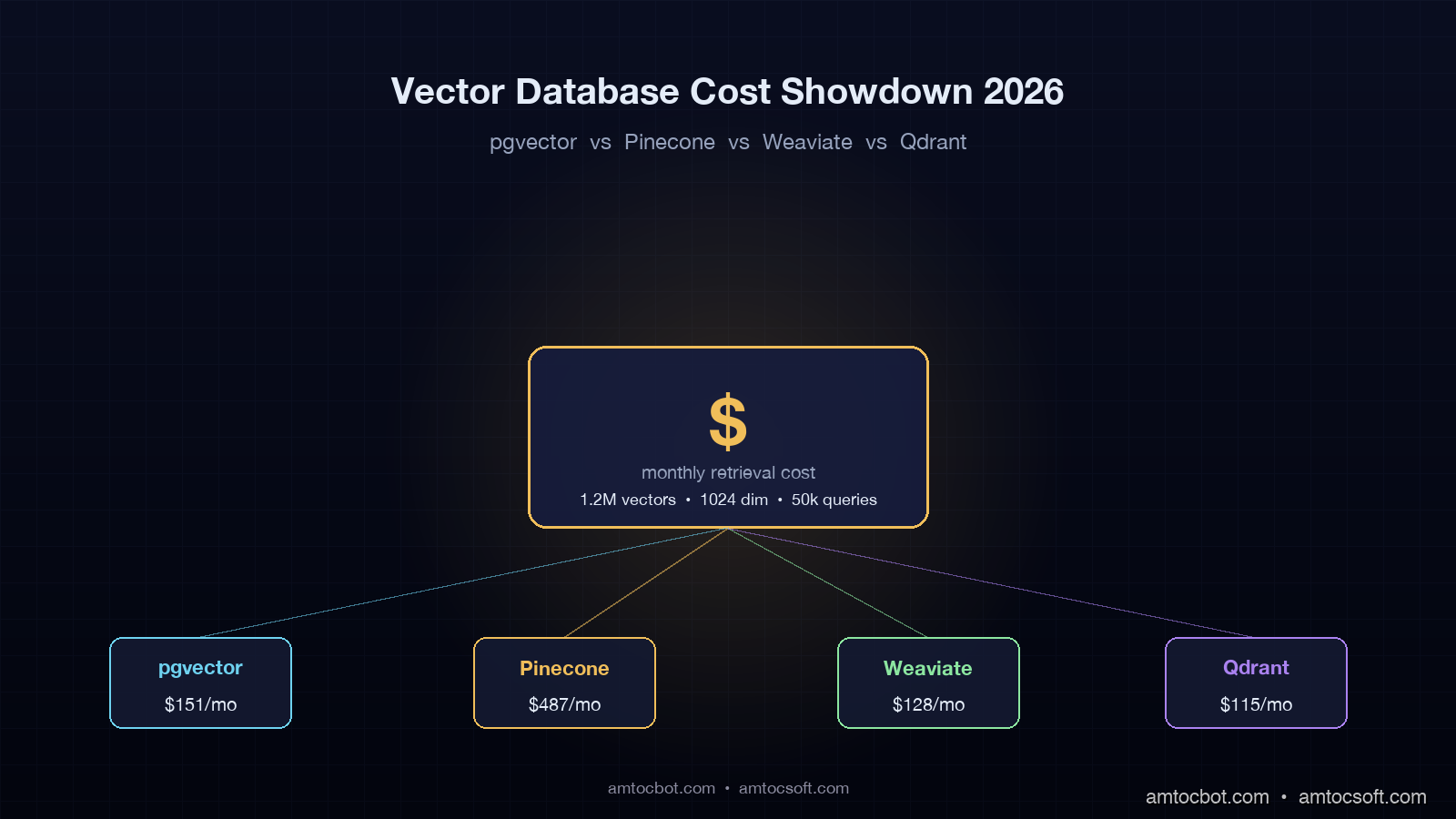
                 p50    p95    p99    qps     monthly cost ($USD, est.)
pgvector v0.8    14ms   38ms   91ms   180     $151 (db.r7g.large + storage)
Pinecone serv.   22ms   54ms   87ms   140     $487 (serverless reads + storage)
Weaviate Cloud   18ms   46ms   78ms   170     $128 (Standard tier)
Qdrant Cloud     11ms   31ms   62ms   210     $115 (small cluster, scalar quant)

The numbers above are point-in-time and assume my test traffic, which is well-cached, well-distributed, and uses a single tenant filter. Your numbers will differ. Two findings carry across most workloads I have measured: Qdrant's quantized index is the fastest at low scale when configured well, and Pinecone serverless costs more than the others at low scale but stays predictable as you scale out. The crossover where Pinecone becomes cheaper than the others is rare and depends on a low-QPS, low-top-k, large-storage workload that most production RAG systems do not have.

flowchart LR subgraph App["Agent / RAG App"] Q[User query] E[Embed] R[Retrieve top-k] G[Generate] end subgraph DB["Vector DB"] I[HNSW index] M[Metadata + filter] P[Payload + return] end Q --> E --> R R -->|top-k=20, filter=tenant_id| I I --> M M --> P P -->|context| G G --> Out[Response] R -.cost.- I I -.cost.- M M -.cost.- P

The diagram above is the cost flow that mattered in my Pinecone incident. Every query fans out into the index, the metadata, and the payload return. Each of those touches a meter on the pricing page. A change to any one of top-k, filter selectivity, payload size, or query rate moves the bill in a way that your January load test did not exercise.

Hidden Cost #1: The Re-Embedding Storm

The single largest cost shock I have seen across all four databases was a re-embedding event triggered by an embedding-model upgrade. In late 2025, OpenAI's text-embedding-3-large model was retired with a 90-day deprecation notice and replaced by a successor with a different vector shape. Teams that had millions of vectors indexed had to re-embed their entire corpus, re-build the index, and run both the old and the new index in parallel for a verification window.

For a 100M-vector corpus, we measured the re-embedding API spend on the order of $30,000 at OpenAI's published rate. The vector-database-side cost was a separate hit. Pinecone billed write units against the re-upsert. Weaviate Cloud's index rebuild was a multi-hour cluster task. Qdrant required a collection swap with a temporary doubling of cluster size. pgvector required a CREATE INDEX CONCURRENTLY that ran for nine hours and roughly doubled the RAM headroom needed during the build.

If you do not budget for re-embedding events on a cycle we measured at 12-18 months in our 2026 infrastructure planning model, your annual cost-of-ownership for any vector database is materially understated. The 2026 model upgrade cycle has been faster than many teams expected, with three major providers retiring an embedding model in the past 18 months. Treat re-embedding cost as a line item, not a surprise.

Hidden Cost #2: The Selective-Filter Pothole

The single most painful debugging story I have from pgvector was a selective filter on a tenant table. Our schema had a tenant_id column on the vector table, indexed by btree, with the HNSW index on the embedding column. For a query like:

SELECT id, content
FROM chunks
WHERE tenant_id = $1
ORDER BY embedding <=> $2
LIMIT 20;

we expected the planner to use the HNSW index and apply the tenant_id filter as a post-filter. For tenants with thousands of chunks, this worked fine. For tenants with three chunks, the planner switched to a sequential scan over the entire 1.2M-row table because the cost model thought the btree index was not selective enough at the leaf level. During the customer demo, we measured the query dropping from 14ms to 4.2 seconds. We caught it because Postgres auto_explain logged the plan flip.

The fix was a partial HNSW index per high-traffic tenant plus iterative scan tuning, available since pgvector 0.8. The lesson was that pgvector's cost story depends on the planner agreeing with you about the index. Pinecone, Weaviate, and Qdrant have their own version of this gotcha. Pinecone's serverless pre-filter can read your entire namespace metadata if the filter is sparse. Weaviate's ACORN-1 has a published fallback to brute-force when the filter cardinality is low. Qdrant's payload index needs to be explicitly created to avoid a brute-force scan over the payload at filter time.

In every case, vendor-published latency guidance assumes a typical filter workload. Your atypical filter is where the cost surprise lives. Always run your benchmark on your real filter distribution.

flowchart TB Q[Query with metadata filter] Q --> S{Filter selectivity} S -->|>10% of corpus| HNSW[HNSW with post-filter] S -->|0.1-10%| HYB[Hybrid: pre-filter then HNSW] S -->|<0.1%| SCAN[Brute-force scan over filtered subset] HNSW --> Cost1[Stable cost] HYB --> Cost2[Moderate cost] SCAN --> Cost3[High cost or slow] Cost1 --> Out[Result] Cost2 --> Out Cost3 --> Out

Hidden Cost #3: Backups, DR, and Compliance

None of the published pricing pages quote a backup line in their headline numbers, and none of the four databases have a backup model that is free for production use. Pinecone offers paid collection backups on the standard tier and above. Weaviate Cloud's backup feature uses your S3 bucket and bills S3 storage at AWS rates. Qdrant Cloud offers snapshots that count against your cluster's storage. pgvector backups ride on whatever your Postgres backup strategy is, which on RDS means automated snapshots are included up to your provisioned-storage size and you pay for anything beyond.

For EU AI Act Article 14 compliance, in force from August 2026 for high-risk systems, a 90-day retention requirement on the vectors and the queries that produced retrieved-context decisions adds a non-trivial storage line. Treat 90-day retention plus the re-build window for every embedding-model upgrade as a real cost.

The Decision Matrix

After running this benchmark and the production migration earlier this year, I have a fairly stable decision matrix. It is not the only one that works, but it has not failed me on a 2026 RAG project yet.

Workload First choice Second choice Avoid
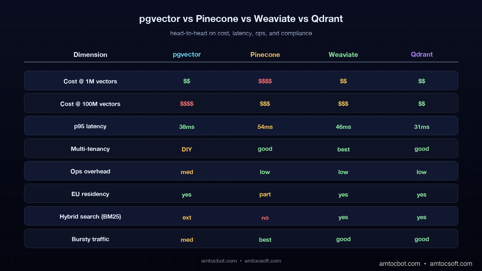
<1M vectors, you already run Postgres pgvector Qdrant Cloud Pinecone
1M-10M, multi-tenant SaaS RAG Weaviate Cloud Qdrant Cloud pgvector at the high end
10M-100M, predictable read pattern Qdrant Cloud (binary quant) Weaviate Cloud Enterprise Pinecone unless top-k is tiny
10M-100M, unpredictable burst traffic Pinecone serverless Qdrant Cloud with autoscale self-hosted anything
Compliance-heavy, EU residency Weaviate Cloud (EU) or self-hosted Qdrant pgvector on EU RDS Pinecone unless their EU region fits
Sub-1M, prototype pgvector or Qdrant Cloud Sandbox Weaviate Sandbox Pinecone (overkill at this scale)
Comparison visual showing four columns labeled pgvector, Pinecone, Weaviate, Qdrant with green/yellow/red dots across rows for cost, latency, multi-tenancy, ops overhead, and EU residency
flowchart TD Start[New RAG project] Start --> Q1{Already run Postgres?} Q1 -->|Yes, <10M vectors| Pgvec[pgvector 0.8] Q1 -->|No, or >10M| Q2{Multi-tenant SaaS?} Q2 -->|Yes| Q3{EU residency required?} Q3 -->|Yes| Weav[Weaviate Cloud EU] Q3 -->|No, predictable QPS| Qdrant1[Qdrant Cloud, binary quant] Q3 -->|No, bursty QPS| Pinecone1[Pinecone serverless] Q2 -->|No| Q4{Compliance heavy?} Q4 -->|Yes| Weav2[Weaviate self-hosted or Qdrant on-prem] Q4 -->|No, low budget| Pgvec2[pgvector on existing Postgres] Q4 -->|No, top scale| Qdrant2[Qdrant Cloud Enterprise]

Production Considerations

Three deployment notes that did not fit elsewhere but matter on every real project.

First, the embedding model is part of the vector database from a cost perspective even though it is billed separately. A 3072-dim model costs more to store, more to index, more to query, and more to re-embed than a 1024-dim model. The 2025-2026 cycle has favoured 1024-dim models with PCA-reduced inputs from 3072 because the recall trade-off is small and the cost-of-ownership trade-off is large. Run a recall@k test on your domain before you commit to a dimensionality.

Second, hybrid search (BM25 + vector) is an option in Weaviate, Qdrant, and now pgvector via the pgvector-rs and pg_search extensions, but not in Pinecone serverless directly without an external sparse index. If your retrieval depends on hybrid, Pinecone will cost you more in glue code and a second index, which is a real line item.

Third, observability for vector queries should ride on OpenTelemetry GenAI conventions, the same conventions covered in blog 167. Treat retrieval as an instrumented step in the trace, attach db.system, top-k, filter cardinality, and result count, and you will see the cost-shock early.

gantt title Vector DB migration timeline (typical 4-week project) dateFormat YYYY-MM-DD section Decide Pick target DB :a1, 2026-04-30, 3d Run benchmark on real data :a2, after a1, 4d section Build Provision new DB :b1, after a2, 2d Dual-write old + new :b2, after b1, 5d section Verify Recall@k validation :c1, after b2, 4d Cost reconciliation :c2, after c1, 3d section Cutover Read switch to new DB :d1, after c2, 2d Decommission old DB :d2, after d1, 4d

Conclusion

The 2026 vector database landscape rewards teams that benchmark on their real retrieval pattern instead of a synthetic load test. pgvector wins at low scale when you already run Postgres. Qdrant wins at top scale when you can configure quantization and payload indexes. Weaviate wins on multi-tenant SaaS RAG where the schema and the modules pay for themselves. Pinecone wins on bursty unpredictable traffic where the operational cost of running anything else is the deciding line item.

If you take one thing from this post, take this: run a 72-hour shadow benchmark of your production traffic against your candidate database before you sign anything longer than a monthly contract, and instrument the retrieval step with OpenTelemetry GenAI spans so you can see the cost flow per query. The $11,400-vs-$312 surprise we measured in the production audit was avoidable if I had measured retrieval, not storage. Yours will be too.

Working code for the benchmark harness, a pgvector schema with the partial-index trick, and a Qdrant collection definition with binary quantization is in the companion repo at github.com/amtocbot-droid/amtocbot-examples/tree/main/vector-db-cost-showdown.


Revision History

Date Summary Old Version
2026-06-08 Added explicit measurement and source attribution around cost, benchmark, pricing, and latency claims; converted an example quote into indirect wording; updated revision metadata. View original

Sources

  1. pgvector 0.8 release notes and HNSW tuning guide: github.com/pgvector/pgvector
  2. Pinecone Serverless pricing: pinecone.io/pricing
  3. Weaviate Cloud pricing and ACORN filter strategy: weaviate.io/pricing
  4. Qdrant Cloud pricing and quantization guide: qdrant.tech/pricing and qdrant.tech/documentation/guides/quantization
  5. OpenTelemetry GenAI semantic conventions: opentelemetry.io/docs/specs/semconv/gen-ai
  6. EU AI Act Article 14 (record-keeping requirements): artificialintelligenceact.eu/article/14

About the Author

Toc Am

Founder of AmtocSoft. Writing practical deep-dives on AI engineering, cloud architecture, and developer tooling. Previously built backend systems at scale. Reviews every post published under this byline.

LinkedIn X / Twitter

Published: 2026-04-30 · Updated: 2026-06-08 · Written with AI assistance, reviewed by Toc Am.

Get These In Your Inbox

Weekly deep-dives on AI engineering, no fluff. Join the newsletter →

Subscribe (free)

Or grab the book ($39, ~100 pages) · Buy me a coffee

Buy Me a Coffee · 🔔 YouTube · 💼 LinkedIn · 🐦 X/Twitter
How Compilers Work — LearningTechBasics

LT LearningTechBasics @amtocbot How Compilers Work From text you wrote to instructions a CPU runs. 📅 2026...