Showing posts with label scaling. Show all posts

Monday, April 13, 2026

Kubernetes in Production: What Nobody Tells You About Running K8s at Scale

Kubernetes Production: The hidden complexity behind the YAML

Introduction

The Kubernetes documentation will teach you how to write a Deployment. The tutorials will show you how to expose it with a Service. The YouTube videos will walk you through setting up a local cluster with Minikube. None of them will prepare you for 3am when your cluster autoscaler is not scaling, your nodes are out of capacity, half your pods are in OOMKilled loops, and your on-call engineer is staring at Grafana trying to figure out which of the six different resource limit configurations is lying to them.

Kubernetes has a remarkably well-documented surface. The parts nobody writes about are the operational realities that only become visible when your cluster is running real workloads at real scale: the resource request and limit traps that cause cascading failures, the subtle differences between liveness and readiness probes that turn a single unhealthy pod into a cluster-wide outage, the RBAC anti-patterns that quietly give service accounts more access than they need, and the cost optimization levers that most teams leave untouched until their cloud bill reaches a number that cannot be ignored.

This post is a collection of hard-won production knowledge. It is written for engineers who understand Kubernetes fundamentals — they can write Deployments, Services, and ConfigMaps — and want to understand what it actually means to run Kubernetes responsibly at scale. We will cover resource management, autoscaling architectures, pod scheduling, disruption budgets, probe configuration, secrets and ConfigMap rotation, network policy fundamentals, and real incident scenarios with their root causes and fixes.

This is not the documentation. This is what happens after you follow the documentation.


Resource Requests and Limits: The OOMKilled Trap

Of all the Kubernetes configuration mistakes that cause production incidents, the most common by a wide margin is incorrect resource requests and limits. The confusing part is that the documentation explains the mechanics clearly — the damage comes from not understanding the downstream effects.

What Requests and Limits Actually Do

A resource request is a scheduling hint. The Kubernetes scheduler places your pod on a node that has at least that much CPU and memory available. Once the pod is running, the request does not enforce anything — a pod with a 100m CPU request can use 4000m CPU if the node has spare capacity.

A resource limit is an enforcement boundary. CPU limits are implemented via Linux cgroups and result in CPU throttling when a container exceeds its limit. Memory limits are enforced strictly: when a container exceeds its memory limit, it is killed immediately with an OOMKilled exit code. The pod will restart (per its restart policy), hit the memory limit again, restart again, and enter a CrashLoopBackOff death spiral.

This asymmetry is the source of most production resource incidents:

CPU Memory
Exceeds request Allowed (uses spare capacity) Allowed
Exceeds limit Throttled (slows down) Killed immediately
Effect Performance degradation Pod restart / crash loop
Detection High throttle ratio in metrics OOMKilled in pod events

The Three Anti-Patterns

Anti-pattern 1: Memory limit = memory request. Setting requests.memory: "512Mi" and limits.memory: "512Mi" looks clean and predictable. In practice, many applications have unpredictable memory usage — a JVM application's memory usage includes heap, metaspace, direct memory, and thread stacks, all of which fluctuate. Setting the limit exactly equal to the request means any spike above your estimated steady-state usage kills the container. Instead, set the limit 1.5x to 2x the request for applications with variable memory usage, and monitor actual memory usage to tune both over time.

Anti-pattern 2: No requests set at all. Without resource requests, all your pods land in the BestEffort QoS class. Kubernetes will evict BestEffort pods first when a node is under memory pressure. This means your application silently disappears when any node gets busy — no alerts, no CrashLoopBackOff, just pods gone. Always set at least memory requests on every container.

Anti-pattern 3: CPU limits in latency-sensitive services. CPU limits are implemented via CFS (Completely Fair Scheduler) bandwidth control. At high request rates, CPU throttling introduces latency spikes that are difficult to diagnose because the application's CPU usage metrics look fine (they show utilization, not throttle time). For latency-sensitive services, consider setting CPU requests without CPU limits — this gives the scheduler accurate placement information while allowing bursting. Monitor container_cpu_cfs_throttled_seconds_total to detect throttling.

# Good resource configuration for a latency-sensitive API
resources:
  requests:
    memory: "256Mi"   # Conservative estimate — scheduler uses this
    cpu: "200m"       # Accurate estimate — affects scheduling quality
  limits:
    memory: "512Mi"   # 2x request — room for GC spikes, caching, etc.
    # No CPU limit — avoids throttle-induced latency spikes
    # Monitor cpu_cfs_throttled_seconds if you add one later
# Good resource configuration for a batch/background worker
resources:
  requests:
    memory: "512Mi"
    cpu: "500m"
  limits:
    memory: "1Gi"     # 2x request
    cpu: "2000m"      # Limit is acceptable for batch — latency is less critical

Diagnosing Resource Problems in Production

# Check which pods are being OOMKilled
kubectl get pods -A | grep -i oom
kubectl get events -A | grep OOMKill

# Check actual memory usage vs limits (requires metrics-server)
kubectl top pods -A --sort-by=memory

# Check CPU throttle ratio (requires Prometheus)
# High values (>0.25) indicate CPU limit is too low
rate(container_cpu_cfs_throttled_seconds_total[5m]) /
rate(container_cpu_cfs_periods_total[5m])

# Find pods with no resource requests (BestEffort QoS)
kubectl get pods -A -o json | jq -r '
  .items[] |
  select(.spec.containers[].resources.requests == null) |
  "\(.metadata.namespace)/\(.metadata.name)"
'

Autoscaling: HPA vs VPA vs KEDA

Kubernetes provides three autoscaling mechanisms that operate at different layers. Understanding when to use each — and how they interact — is essential for cost-efficient, reliable production deployments.
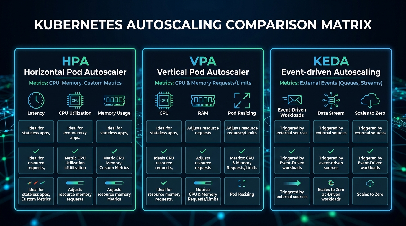
Kubernetes Autoscaling: HPA vs VPA vs KEDA decision matrix

HPA: Horizontal Pod Autoscaler

HPA adds or removes pod replicas based on observed metrics. It is the right tool when your workload can be horizontally distributed (stateless APIs, workers) and when traffic varies significantly over time.

# hpa.yaml — scale based on CPU and custom metrics simultaneously
apiVersion: autoscaling/v2
kind: HorizontalPodAutoscaler
metadata:
  name: api-service-hpa
  namespace: production
spec:
  scaleTargetRef:
    apiVersion: apps/v1
    kind: Deployment
    name: api-service
  minReplicas: 3          # Never go below 3 — one per AZ minimum
  maxReplicas: 50
  metrics:
    # Primary: CPU utilization
    - type: Resource
      resource:
        name: cpu
        target:
          type: Utilization
          averageUtilization: 70   # Scale up when average CPU hits 70%
    # Secondary: custom metric from Prometheus
    - type: Pods
      pods:
        metric:
          name: http_requests_per_second
        target:
          type: AverageValue
          averageValue: "1000"     # 1000 req/s per pod before scaling up
  behavior:
    scaleUp:
      stabilizationWindowSeconds: 60    # Wait 60s before scaling up again
      policies:
        - type: Pods
          value: 4                       # Add at most 4 pods at a time
          periodSeconds: 60
    scaleDown:
      stabilizationWindowSeconds: 300   # Wait 5 min before scaling down — avoid flapping
      policies:
        - type: Percent
          value: 10                      # Remove at most 10% of pods per minute
          periodSeconds: 60

HPA gotcha: HPA reads resource metrics from the metrics-server (for CPU/memory) or from a custom metrics adapter (for Prometheus metrics). If the metrics-server is unavailable or slow, HPA stops scaling. Always monitor your metrics-server's availability, and make sure it has enough resources — it is a critical path component for autoscaling.

VPA: Vertical Pod Autoscaler

VPA adjusts CPU and memory requests automatically based on observed usage, rather than adding replicas. It is useful for singleton services (databases, stateful sets), batch jobs, and any workload where you do not know the right resource requests at deployment time.

VPA has three operating modes:

  • Off (recommendation mode): VPA calculates recommendations but does not apply them. Useful for right-sizing existing deployments.
  • Initial: VPA only sets resources when a pod is first created. Existing pods are not affected.
  • Auto: VPA evicts and recreates pods to apply new resource recommendations. This causes pod restarts.
# vpa.yaml — recommendation mode for right-sizing
apiVersion: autoscaling.k8s.io/v1
kind: VerticalPodAutoscaler
metadata:
  name: api-service-vpa
  namespace: production
spec:
  targetRef:
    apiVersion: apps/v1
    kind: Deployment
    name: api-service
  updatePolicy:
    updateMode: "Off"   # Recommendation only — inspect with kubectl describe vpa
  resourcePolicy:
    containerPolicies:
      - containerName: api-service
        minAllowed:
          memory: "128Mi"
          cpu: "50m"
        maxAllowed:
          memory: "2Gi"
          cpu: "4000m"
        controlledResources: ["cpu", "memory"]

Important: Do not run HPA and VPA in Auto mode on the same deployment for the same metrics. HPA and VPA can conflict — VPA wants to resize pods while HPA wants to scale replicas, leading to thrashing. The safe combination: HPA on CPU/custom metrics for scaling replicas, VPA in Off mode for right-sizing recommendations that you apply manually.

KEDA: Kubernetes Event-Driven Autoscaling

KEDA extends HPA to scale based on event sources — Kafka consumer group lag, RabbitMQ queue depth, AWS SQS queue length, Prometheus queries, cron schedules, and 50+ other scalers. Critically, KEDA can scale to zero, which HPA cannot do.

# keda-scaledobject.yaml — scale workers based on Kafka lag
apiVersion: keda.sh/v1alpha1
kind: ScaledObject
metadata:
  name: kafka-consumer-scaler
  namespace: production
spec:
  scaleTargetRef:
    apiVersion: apps/v1
    kind: Deployment
    name: order-processor
  minReplicaCount: 0    # Scale to zero when queue is empty — saves cost
  maxReplicaCount: 20
  pollingInterval: 15   # Check every 15 seconds
  cooldownPeriod: 300   # Wait 5 min before scaling down after queue drains
  triggers:
    - type: kafka
      metadata:
        bootstrapServers: kafka-broker:9092
        consumerGroup: order-processors
        topic: orders
        lagThreshold: "100"      # One worker per 100 messages of lag
        offsetResetPolicy: latest

KEDA is the right choice for:
- Queue/event-driven consumers where idle capacity is pure waste
- Batch workloads with predictable schedules (cron-based scaling)
- Any workload where true scale-to-zero makes economic sense


Pod Scheduling: Affinity, Anti-Affinity, and Disruption Budgets

Why Anti-Affinity Is Not Optional for Production

If you run three replicas of a critical service and all three land on the same node, your "three-replica HA setup" is actually a single point of failure. Node hardware failure, kernel panic, or a bad kubectl drain wipes all three pods simultaneously.

# Pod anti-affinity: spread pods across availability zones
spec:
  affinity:
    podAntiAffinity:
      # Hard rule: never schedule two pods of this app on the same AZ
      requiredDuringSchedulingIgnoredDuringExecution:
        - labelSelector:
            matchLabels:
              app: api-service
          topologyKey: topology.kubernetes.io/zone
      # Soft rule: prefer different nodes within an AZ
      preferredDuringSchedulingIgnoredDuringExecution:
        - weight: 100
          podAffinityTerm:
            labelSelector:
              matchLabels:
                app: api-service
            topologyKey: kubernetes.io/hostname

In 2026, topologySpreadConstraints is the preferred approach over pod anti-affinity for most use cases — it gives you more precise control:

# Topology spread: distribute pods evenly across zones and nodes
spec:
  topologySpreadConstraints:
    # Spread across availability zones
    - maxSkew: 1                          # At most 1 more pod in any zone than others
      topologyKey: topology.kubernetes.io/zone
      whenUnsatisfiable: DoNotSchedule    # Hard requirement
      labelSelector:
        matchLabels:
          app: api-service
    # Also spread across individual nodes
    - maxSkew: 2                          # Allow up to 2 more pods on any node
      topologyKey: kubernetes.io/hostname
      whenUnsatisfiable: ScheduleAnyway   # Soft preference
      labelSelector:
        matchLabels:
          app: api-service

Pod Disruption Budgets: Your Last Line of Defense

A PodDisruptionBudget (PDB) defines the minimum number of pods that must remain available during voluntary disruptions — node drains for maintenance, cluster upgrades, and kubectl drain operations. Without a PDB, kubectl drain will evict all pods from a node simultaneously, potentially taking your entire service offline during what should be a routine maintenance operation.

# pdb.yaml — always configure this for production workloads
apiVersion: policy/v1
kind: PodDisruptionBudget
metadata:
  name: api-service-pdb
  namespace: production
spec:
  # Require that at least 2 pods are always available
  # For a 3-replica deployment, this means at most 1 can be disrupted at a time
  minAvailable: 2
  # Alternative: maxUnavailable: 1  (same result for 3 replicas, more flexible for HPA)
  selector:
    matchLabels:
      app: api-service

PDB gotcha: If your HPA scales down to minReplicas and your PDB requires minAvailable: 2, the PDB will block node drains because there is no slack. Either set minAvailable as a percentage (minAvailable: "50%") or ensure your HPA minReplicas is always greater than your minAvailable count.


Probes: The Configuration Mistakes That Cause Outages

The three Kubernetes probe types — liveness, readiness, and startup — are conceptually simple but operationally treacherous. Misconfiguring them is one of the most common causes of self-inflicted production incidents.

flowchart TD A[Pod starts] --> B[Startup probe runs\nuntil success or failure] B -->|Success| C[Liveness + Readiness probes\nbegin running concurrently] B -->|failureThreshold exceeded| D[Container killed\nand restarted] C --> E{Liveness probe} C --> F{Readiness probe} E -->|Pass| G[Container stays alive] E -->|failureThreshold exceeded| H[Container killed\nand restarted — restart count++] F -->|Pass| I[Pod in Ready state\nreceives traffic from Service] F -->|Fail| J[Pod removed from\nService endpoints\nno new traffic routed] J -->|Recovery| I H --> A style D fill:#c1121f,color:#fff style H fill:#c1121f,color:#fff style I fill:#2d6a4f,color:#fff style J fill:#e76f51,color:#fff

The Three Probes and Their Distinct Roles

Liveness probe: Answers "Is this container alive and worth keeping?" A failing liveness probe causes the container to be killed and restarted. Use this for detecting deadlocks and zombie states — conditions where the application process is running but cannot make progress and will never recover on its own. Do NOT use the liveness probe to check upstream dependencies (databases, caches). If your database goes down, failing the liveness probe causes all your pods to restart in a loop, turning a recoverable database outage into a full application outage.

Readiness probe: Answers "Is this container ready to accept traffic?" A failing readiness probe removes the pod from Service endpoints so no new requests are routed to it, but the container is not killed. Use this to signal that the application is warming up (loading caches, establishing connection pools, processing a backlog), or that it is temporarily overwhelmed and wants to stop receiving new traffic. It is appropriate to check upstream dependencies in the readiness probe.

Startup probe: Answers "Has this container finished starting up?" It runs exclusively until it succeeds (after which the liveness and readiness probes begin). It is essential for slow-starting applications (JVM applications, applications loading large ML models) where you need generous startup time without making the liveness probe's failureThreshold so high that it delays detection of runtime failures.

# Well-configured probes for a Node.js API
livenessProbe:
  httpGet:
    path: /health/live    # Returns 200 if process is running and not deadlocked
    port: 3000            # Does NOT check database connectivity
  initialDelaySeconds: 30 # Grace period after container starts
  periodSeconds: 10
  timeoutSeconds: 5
  failureThreshold: 3     # Kill after 3 consecutive failures (30s window)

readinessProbe:
  httpGet:
    path: /health/ready   # Returns 200 only if DB connection is healthy,
    port: 3000            # cache is warm, and service is accepting load
  initialDelaySeconds: 10
  periodSeconds: 5
  timeoutSeconds: 3
  failureThreshold: 3     # Stop receiving traffic after 3 failures (15s)
  successThreshold: 2     # Require 2 consecutive passes before re-adding to LB

startupProbe:
  httpGet:
    path: /health/live
    port: 3000
  failureThreshold: 30    # 30 attempts × 10s = 5 minutes for startup
  periodSeconds: 10

The corresponding health check implementation in Node.js:

// health.js — production-grade health check implementation
const express = require('express');
const router = express.Router();

// Liveness: is the process alive and responsive?
// Keep this CHEAP and independent of external dependencies.
router.get('/health/live', (req, res) => {
  // Check for internal deadlock indicators
  const memUsage = process.memoryUsage();
  const heapUsedMB = memUsage.heapUsed / 1024 / 1024;

  // Fail liveness if heap usage is suspiciously high (possible memory leak)
  if (heapUsedMB > 1800) { // 1.8GB — approaching our 2GB limit
    return res.status(503).json({
      status: 'unhealthy',
      reason: 'heap_near_limit',
      heapUsedMB: Math.round(heapUsedMB)
    });
  }

  res.json({ status: 'alive', uptime: process.uptime() });
});

// Readiness: is the service ready to accept requests?
// Check external dependencies here — it is safe to do so.
router.get('/health/ready', async (req, res) => {
  const checks = await Promise.allSettled([
    checkDatabase(),
    checkRedisConnection(),
    checkWarmupComplete()
  ]);

  const allHealthy = checks.every(c => c.status === 'fulfilled' && c.value === true);

  if (!allHealthy) {
    const failures = checks
      .map((c, i) => ({ name: ['database', 'redis', 'warmup'][i], ok: c.status === 'fulfilled' }))
      .filter(c => !c.ok)
      .map(c => c.name);

    return res.status(503).json({ status: 'not_ready', failing: failures });
  }

  res.json({ status: 'ready' });
});

// Internal: check if cache warmup is complete
let warmupComplete = false;
async function runWarmup() {
  // Load frequently-accessed data into memory cache
  await prefetchTopCategories();
  await prefetchConfigFromDB();
  warmupComplete = true;
  console.log('Warmup complete — pod is now ready');
}

function checkWarmupComplete() {
  return Promise.resolve(warmupComplete);
}

runWarmup(); // Run on startup — readiness probe will fail until complete

ConfigMap and Secret Rotation Without Restarts

A frustrating default Kubernetes behavior: when you update a ConfigMap or Secret, pods that have mounted them as volumes will see the updated values on disk within ~60 seconds (the kubelet's sync interval). But pods using envFrom or individual env.valueFrom.secretKeyRef entries will never see the updated values without a pod restart.

For most configuration, this is fine — you trigger a rolling restart as part of the deploy. But for secrets that rotate automatically (TLS certificates, database credentials rotated by AWS Secrets Manager), requiring a pod restart every time a secret rotates is operationally painful and can cause brief unavailability.

Pattern 1: Volume Mounts for Rotating Secrets

Mount the Secret as a volume instead of injecting it as an environment variable. The application reads the file at runtime, detecting changes and reloading without restart:

spec:
  containers:
  - name: api-service
    volumeMounts:
    - name: db-credentials
      mountPath: /etc/secrets/db
      readOnly: true
  volumes:
  - name: db-credentials
    secret:
      secretName: db-credentials
      # Optional: set defaultMode to restrict file permissions
      defaultMode: 0400
// Reload credentials from file on each connection (not just at startup)
const fs = require('fs');

function getDatabaseCredentials() {
  // Read fresh credentials on every pool creation
  // This handles automatic secret rotation gracefully
  const creds = JSON.parse(
    fs.readFileSync('/etc/secrets/db/credentials.json', 'utf8')
  );
  return {
    host: creds.host,
    username: creds.username,
    password: creds.password,  // Picks up rotated password automatically
    database: creds.database
  };
}

Pattern 2: Reloader for Environment Variable Secrets

For applications that cannot easily reload configuration at runtime, Reloader is a Kubernetes controller that watches ConfigMaps and Secrets and triggers rolling restarts of Deployments when they change:

# Deployment with Reloader annotation
apiVersion: apps/v1
kind: Deployment
metadata:
  name: api-service
  annotations:
    # Trigger rolling restart when this specific Secret changes
    secret.reloader.stakater.com/reload: "api-service-secrets"
    # Or: trigger on ANY configmap/secret change
    reloader.stakater.com/auto: "true"

RBAC Patterns: Least Privilege at Scale

graph LR subgraph "Team: Backend" SA1[ServiceAccount:\napi-service] --> CR1[ClusterRole:\nread-own-pods] U1[Developer Alice] --> R1[Role:\nbackend-developer\nnamespace: backend] end subgraph "Team: Platform" SA2[ServiceAccount:\nargocd-controller] --> CR2[ClusterRole:\napp-deployer] U2[Platform Engineer Bob] --> CR3[ClusterRole:\nplatform-admin] end subgraph "Restricted" CR3 -->|can NOT| S[cluster-admin\nClusterRole] end style S fill:#c1121f,color:#fff style CR3 fill:#1a4e8a,color:#fff

The most dangerous RBAC mistake in Kubernetes is giving workloads cluster-admin or overly broad permissions "to make it work." A compromised pod with cluster-admin can read all Secrets, delete all Deployments, and create new privileged pods across the entire cluster.

Follow these RBAC rules in production:

Rule 1: Namespace-scoped Roles, not ClusterRoles, for application service accounts. Most application workloads only need to read their own ConfigMaps or create Jobs in their own namespace. Use Role (namespace-scoped) rather than ClusterRole (cluster-wide).

Rule 2: Never bind cluster-admin to a service account. If a controller genuinely needs cluster-wide access (ArgoCD, cert-manager, the cluster autoscaler), create a minimal ClusterRole with exactly the resources and verbs required.

Rule 3: Audit all ServiceAccount token mounts. By default, Kubernetes mounts a ServiceAccount token into every pod at /var/run/secrets/kubernetes.io/serviceaccount/token. For pods that do not need to call the Kubernetes API at all, set automountServiceAccountToken: false.

# Minimal RBAC for an application that only reads its own ConfigMaps
apiVersion: v1
kind: ServiceAccount
metadata:
  name: api-service
  namespace: production
automountServiceAccountToken: false  # Disable default token mount
---
apiVersion: rbac.authorization.k8s.io/v1
kind: Role
metadata:
  name: api-service-role
  namespace: production
rules:
  - apiGroups: [""]
    resources: ["configmaps"]
    resourceNames: ["api-service-config"]  # Scope to specific resource by name
    verbs: ["get", "watch"]
---
apiVersion: rbac.authorization.k8s.io/v1
kind: RoleBinding
metadata:
  name: api-service-binding
  namespace: production
subjects:
  - kind: ServiceAccount
    name: api-service
    namespace: production
roleRef:
  kind: Role
  name: api-service-role
  apiGroup: rbac.authorization.k8s.io

Cost Optimization: Spot Nodes and the Cluster Autoscaler

Running Kubernetes on cloud-managed clusters (EKS, GKE, AKS) without cost optimization can be expensive. The most impactful levers are spot/preemptible instances and the Cluster Autoscaler.

Mixed Instance Groups with Spot Nodes

On AWS EKS, a common pattern is to use two node groups:
- On-demand group (small): 2-3 nodes, always running, for critical system components (monitoring, ingress controllers, GitOps controllers)
- Spot group (large): scales from 0 to many nodes, for application workloads

This architecture can reduce EC2 costs by 60-80% for variable workloads. The key is making your application pods tolerate spot interruptions gracefully:

# Deployment tolerating spot nodes with graceful disruption handling
spec:
  template:
    spec:
      # Allow scheduling on spot nodes
      tolerations:
        - key: "spot-instance"
          operator: "Equal"
          value: "true"
          effect: "NoSchedule"
      # Prefer spot nodes but fall back to on-demand
      affinity:
        nodeAffinity:
          preferredDuringSchedulingIgnoredDuringExecution:
            - weight: 90
              preference:
                matchExpressions:
                  - key: node-lifecycle
                    operator: In
                    values: ["spot"]
      # Give pods 60 seconds to finish in-flight requests on spot interruption
      terminationGracePeriodSeconds: 60
  strategy:
    rollingUpdate:
      maxUnavailable: 1     # Never take more than 1 pod offline during disruption
      maxSurge: 2           # Allow 2 extra pods during rollout for fast replacement

Real Incident Scenarios

Incident 1: The Silent OOMKill Loop
Symptoms: API response rate drops 40% during peak traffic. No errors in application logs. Pod restart count climbs steadily.
Root cause: Memory limit was set at 256Mi based on startup measurements. Under peak load, the Node.js heap grew to 280Mi during a cache miss storm. Pods were being OOMKilled every 8-12 minutes, just infrequently enough that no alert fired, but frequently enough to significantly impact capacity.
Fix: Doubled memory limit to 512Mi. Added container_oom_events_total alert. Added heap size telemetry to application metrics.

Incident 2: The Readiness Probe Cascade
Symptoms: During a database maintenance window, 100% of API pods became unavailable within 60 seconds. Load balancer returned 503 to all traffic.
Root cause: The liveness probe (not readiness) was checking database connectivity. When the database went into maintenance mode, liveness probes failed, Kubernetes restarted all pods, the new pods immediately failed their liveness probes, and the restart loop prevented any pods from reaching Running state.
Fix: Separated liveness (process health only) from readiness (dependency health). Database connectivity check moved to readiness probe only. Liveness probe reduced to checking an in-process health flag.

Incident 3: The Node Drain Outage
Symptoms: Routine EKS node version upgrade caused a 90-second full outage of the payments service.
Root cause: kubectl drain evicted all three payment service pods simultaneously. No PDB was configured. The rolling restart of the Deployment took 90 seconds as new pods passed health checks.
Fix: Added PDB with minAvailable: 2. Updated cluster upgrade runbook to validate all critical services have PDBs before any drain operation.


Conclusion

The gap between "running Kubernetes" and "running Kubernetes well in production" is wider than most teams expect. The challenges in this post — resource tuning, autoscaling architecture, probe configuration, RBAC hygiene, secret rotation, and cost optimization — are not edge cases. They are the table stakes for operating a cluster that your organization can rely on.

The pattern that emerges from all of these lessons is the same: Kubernetes defaults are optimized for developer experience and ease of getting started, not for production resilience. Every production cluster needs deliberate configuration to add the safety margins and operational controls that the defaults omit.

Start with the fundamentals: set resource requests and limits on every container, configure all three probe types for every service, add PDBs to everything critical, and implement pod anti-affinity to spread across zones. These four changes alone will make your cluster significantly more resilient than the typical Kubernetes deployment.

Layer in GitOps (covered in the companion post on ArgoCD and Flux), observability with OpenTelemetry, and KEDA-based autoscaling as your operational maturity grows. The investment pays compound returns: every incident you prevent is a production outage your team does not have to debug at 3am.

The best Kubernetes clusters are the boring ones — the ones where nothing exciting ever happens, because every failure mode was anticipated and handled before it could become an incident.


Sources

About the Author

Toc Am

Founder of AmtocSoft. Writing practical deep-dives on AI engineering, cloud architecture, and developer tooling. Previously built backend systems at scale. Reviews every post published under this byline.

LinkedIn X / Twitter

Published: 2026-04-15 · Updated: 2026-04-18 · Written with AI assistance, reviewed by Toc Am.

Get These In Your Inbox

Weekly deep-dives on AI engineering, no fluff. Join the newsletter →

Subscribe (free)

Or grab the book ($39, ~100 pages) · Buy me a coffee

Buy Me a Coffee · 🔔 YouTube · 💼 LinkedIn · 🐦 X/Twitter

Database Scaling in 2026: Read Replicas, Sharding, and the Connection Pooling Crisis

Database Scaling Hero

Introduction

Databases are where most application scaling plans fall apart. Your API tier is stateless and horizontally scalable — adding more containers is straightforward. Your CDN handles static assets globally. Your message queue absorbs traffic spikes. But your database sits at the bottom of the stack, stateful and stubborn, fielding every read and write that every other component eventually needs.

At small scale, a single PostgreSQL instance with 16GB of RAM and fast SSDs handles thousands of requests per second without complaint. But growth is non-linear. Traffic doubles, and your query latency doubles too — because the working set no longer fits in the buffer pool. You add indexes, the writes slow down. You optimize queries, the connection count climbs. One day you hit a wall: 500 open connections, each holding a 2MB memory allocation in PostgreSQL, and your 16GB database server is spending 40% of its resources just managing connections rather than executing queries.

This post is about that wall, and how to get past it. We will cover the three primary database scaling strategies: read replicas for distributing read load, connection pooling for managing the connection multiplexing problem, and sharding for when a single database instance — no matter how powerful — cannot hold all your data or handle all your writes. We will look at real configuration examples for PgBouncer, Python code with psycopg2, and Node.js with pg, and we will walk through the decision framework for knowing when to apply each technique.

By the end of this post, you will have a concrete mental model for diagnosing database scaling bottlenecks and a toolkit of production-grade solutions.


The Problem: How Single-Database Systems Break Under Load

Before reaching for any scaling technique, it helps to understand exactly how and why a single-database architecture fails. There are three distinct failure modes, and they require different solutions.

Failure Mode 1: Read Saturation

The most common failure mode is read saturation. Most production web applications have a read-to-write ratio of 80:20 or higher — sometimes 95:5 for content-heavy sites. Product pages, user profiles, search results, analytics dashboards: all reads. Your database is spending the vast majority of its CPU time serving queries that do not modify any data.

A single PostgreSQL primary can handle substantial read throughput, but it has limits. Sequential scans, hash joins, and sort operations are CPU-intensive. When query parallelism saturates your CPU cores, latency climbs even for simple indexed lookups because queries queue behind long-running analytical queries.

The instinct to "just add an index" only goes so far. Each additional index speeds up reads but slows writes (PostgreSQL must maintain every index on every INSERT, UPDATE, and DELETE). You reach a point where indexing cannot save you and you need physical read capacity — more CPUs, more memory, more disk I/O — which means spreading reads across multiple machines.

Failure Mode 2: The Connection Limit Crisis

PostgreSQL is a process-per-connection database. Each connection spawns a backend process that consumes roughly 5-10MB of RAM just for overhead, before any query data is allocated. With 500 connections, you have 2.5-5GB of RAM consumed by idle processes. With 1,000 connections — a number easily reached by a moderately successful Node.js application with a connection pool per container — you have consumed 10GB of RAM on process overhead alone.

PostgreSQL's default max_connections is 100. Most production deployments raise this to 500 or 1,000, but the problem compounds: at 1,000 connections, PostgreSQL's shared memory structures (particularly the lock tables) start showing contention that degrades throughput for everyone.

The cruel irony is that most of those connections are idle at any given moment. A web server with 100 concurrent users might hold 400 database connections, of which 390 are waiting for the next request to arrive. The connections exist because each application thread or process needs its own. This is the connection multiplexing problem, and it is why connection poolers like PgBouncer exist.

Failure Mode 3: Write Saturation and Storage Limits

The third failure mode is less common but more severe: you outgrow a single machine's write throughput or storage capacity. If you are writing millions of events per second, archiving time-series sensor data, or storing petabytes of user-generated content, even the largest available cloud database instance cannot keep up. This is where sharding becomes unavoidable.

Write saturation manifests as WAL (Write-Ahead Log) throughput limits, replication lag on replicas, and long-running vacuum operations that cannot keep up with the rate of dead tuple accumulation. Storage limits are more obvious: when your dataset exceeds what fits on a single instance, you must partition it.


How It Works: Read Replicas and Replication

Database Replication Architecture

PostgreSQL's built-in streaming replication solves read saturation by maintaining one or more replica instances that stay synchronized with the primary in near-real-time. The primary writes all changes to the WAL (Write-Ahead Log), and replicas stream and apply those WAL records continuously.

The key architectural decision is how your application routes queries. Read replicas are useless if all your application code sends every query to the primary. You need explicit read/write splitting.

flowchart TD APP[Application Tier\nMultiple instances] --> LB[Load Balancer / Connection Router] LB -->|Write queries\nINSERT, UPDATE, DELETE\nDDL| PRIMARY[(Primary\nPostgreSQL\nAll writes)] LB -->|Read queries\nSELECT| REPLICA1[(Replica 1\nStreaming\nReplication)] LB -->|Read queries\nSELECT| REPLICA2[(Replica 2\nStreaming\nReplication)] LB -->|Read queries\nSELECT| REPLICA3[(Replica 3\nStreaming\nReplication)] PRIMARY -->|WAL stream| REPLICA1 PRIMARY -->|WAL stream| REPLICA2 PRIMARY -->|WAL stream| REPLICA3 REPLICA1 -->|Promote to primary\non failover| FAILOVER{Failover\nLogic} style PRIMARY fill:#E74C3C,color:#fff style REPLICA1 fill:#27AE60,color:#fff style REPLICA2 fill:#27AE60,color:#fff style REPLICA3 fill:#27AE60,color:#fff style LB fill:#3498DB,color:#fff style APP fill:#9B59B6,color:#fff

Implementing Read/Write Splitting in Python

Here is a production-ready Python database client that routes reads and writes automatically:

import random
import contextlib
import psycopg2
import psycopg2.pool
from typing import Optional
import logging

logger = logging.getLogger(__name__)


class DatabaseRouter:
    """
    Routes database queries to primary (writes) or replica pool (reads).

    Usage:
        router = DatabaseRouter(primary_dsn, replica_dsns)

        # Writes always go to primary
        with router.write_connection() as conn:
            conn.cursor().execute("INSERT INTO events ...")

        # Reads distributed across replicas
        with router.read_connection() as conn:
            conn.cursor().execute("SELECT * FROM users WHERE ...")
    """

    def __init__(
        self,
        primary_dsn: str,
        replica_dsns: list[str],
        min_connections: int = 2,
        max_connections: int = 10,
    ):
        # Primary pool: used for all writes and transactions that mix reads and writes
        self._primary_pool = psycopg2.pool.ThreadedConnectionPool(
            minconn=min_connections,
            maxconn=max_connections,
            dsn=primary_dsn,
        )

        # One pool per replica, for horizontal read scaling
        self._replica_pools = [
            psycopg2.pool.ThreadedConnectionPool(
                minconn=min_connections,
                maxconn=max_connections,
                dsn=dsn,
            )
            for dsn in replica_dsns
        ] if replica_dsns else []

        logger.info(
            "DatabaseRouter initialized: 1 primary, %d replicas",
            len(self._replica_pools),
        )

    def _get_replica_pool(self) -> Optional[psycopg2.pool.ThreadedConnectionPool]:
        """Select a replica pool using round-robin with random starting point."""
        if not self._replica_pools:
            return None
        # Random selection provides load distribution without coordinated state
        return random.choice(self._replica_pools)

    @contextlib.contextmanager
    def write_connection(self):
        """
        Yield a connection to the primary database.
        The connection is returned to the pool on context exit.
        Always use this for: INSERT, UPDATE, DELETE, DDL, BEGIN transactions.
        """
        conn = self._primary_pool.getconn()
        try:
            yield conn
            conn.commit()
        except Exception:
            conn.rollback()
            raise
        finally:
            self._primary_pool.putconn(conn)

    @contextlib.contextmanager
    def read_connection(self):
        """
        Yield a connection to a replica database.
        Falls back to primary if no replicas are configured.

        IMPORTANT: Only use for pure SELECT queries.
        Any query that needs fresh-off-the-write data should use write_connection()
        to avoid replication lag issues.
        """
        replica_pool = self._get_replica_pool()
        pool = replica_pool if replica_pool else self._primary_pool

        conn = pool.getconn()
        try:
            # Replicas are read-only; set autocommit to avoid
            # "cannot run in a transaction block" errors on read-only connections
            conn.set_session(readonly=True, autocommit=True)
            yield conn
        except Exception:
            # Read-only connections don't need rollback, but reset session state
            conn.set_session(readonly=False, autocommit=False)
            raise
        finally:
            conn.set_session(readonly=False, autocommit=False)
            pool.putconn(conn)

    def close(self):
        """Close all connection pools. Call on application shutdown."""
        self._primary_pool.closeall()
        for pool in self._replica_pools:
            pool.closeall()


# Example usage in a web application
def get_user_profile(router: DatabaseRouter, user_id: int) -> dict:
    """Fetch a user profile — read-only, goes to replica."""
    with router.read_connection() as conn:
        with conn.cursor() as cur:
            cur.execute(
                "SELECT id, username, email, created_at FROM users WHERE id = %s",
                (user_id,)
            )
            row = cur.fetchone()
            if row is None:
                return {}
            return {
                "id": row[0],
                "username": row[1],
                "email": row[2],
                "created_at": row[3].isoformat(),
            }


def update_user_email(router: DatabaseRouter, user_id: int, new_email: str) -> bool:
    """Update user email — write, goes to primary."""
    with router.write_connection() as conn:
        with conn.cursor() as cur:
            cur.execute(
                "UPDATE users SET email = %s, updated_at = NOW() WHERE id = %s",
                (new_email, user_id)
            )
            return cur.rowcount == 1

Replication Lag: The Read Replica Gotcha

Streaming replication is asynchronous by default. When you write to the primary and immediately read from a replica, there is a window (typically 10-100ms, sometimes more under load) where the replica has not yet applied the write. For many workloads this is acceptable. For others — like showing a user their own just-submitted form — it causes bugs that are extremely difficult to reproduce.

The standard solution is read-your-writes consistency: after any write operation, route the subsequent reads for that session to the primary for a short window (typically 1-5 seconds). Here is how to implement this:

import time
from threading import local

# Thread-local storage for tracking recent writes
_thread_local = local()

def mark_recent_write():
    """Call this after every write. Forces reads to primary for 2 seconds."""
    _thread_local.last_write_time = time.monotonic()

def should_use_primary_for_read() -> bool:
    """Returns True if we had a recent write and should read from primary."""
    last_write = getattr(_thread_local, 'last_write_time', 0)
    # 2-second window after any write: go to primary to avoid lag
    return (time.monotonic() - last_write) < 2.0

def get_connection(router: DatabaseRouter, write: bool = False):
    """Smart connection getter that handles read-your-writes consistency."""
    if write or should_use_primary_for_read():
        return router.write_connection()
    return router.read_connection()

Connection Pooling: PgBouncer in Production

The connection crisis described in the Problem section has a well-established solution: PgBouncer, a lightweight connection pooler that sits between your application and PostgreSQL. Instead of your 500 application threads each holding a direct PostgreSQL connection, they all connect to PgBouncer, which maintains a small pool of actual PostgreSQL connections and multiplexes them.

PgBouncer supports three pooling modes:

Mode How it works Use case
Session One server connection per client session Legacy apps that use session-level features (SET, temporary tables)
Transaction Server connection held only during a transaction Most modern web apps — the sweet spot
Statement Server connection released after each statement High-frequency, simple queries; no multi-statement transactions

Transaction pooling is what most teams need. With it, 1,000 application connections can share a pool of 50-100 actual PostgreSQL server connections with almost no loss in throughput, because most connections are idle between requests.

PgBouncer Configuration

Here is a production-grade PgBouncer configuration (pgbouncer.ini):

[databases]
# Route connections from app_user@myapp to the actual PostgreSQL server
# The application connects to PgBouncer on port 6432
myapp = host=postgres-primary port=5432 dbname=myapp

# Separate pool for replicas (optional — some teams run a second PgBouncer)
myapp_read = host=postgres-replica1 port=5432 dbname=myapp

[pgbouncer]
# Listen for client connections
listen_port = 6432
listen_addr = 0.0.0.0

# Authentication mode: md5 is widely compatible, scram-sha-256 is more secure
auth_type = scram-sha-256
auth_file = /etc/pgbouncer/userlist.txt

# Pooling mode: transaction is the best choice for modern web apps
pool_mode = transaction

# Server connection limits
# max_client_conn: how many clients PgBouncer accepts
max_client_conn = 2000
# default_pool_size: how many real PostgreSQL connections per database+user pair
default_pool_size = 50
# min_pool_size: keep at least this many connections warm
min_pool_size = 10
# reserve_pool_size: extra connections for bursts
reserve_pool_size = 10
# reserve_pool_timeout: wait this many seconds before using reserve pool
reserve_pool_timeout = 5.0

# Connection limits per database
max_db_connections = 100

# Timeouts
server_idle_timeout = 600      # Close idle server connections after 10 min
client_idle_timeout = 0        # Never close idle client connections (app manages this)
server_connect_timeout = 15    # Fail fast if PostgreSQL is unreachable
query_timeout = 0              # No query timeout at pooler level (set in app)
query_wait_timeout = 120       # Client waits max 2 min for a free server connection

# Performance
server_reset_query = DISCARD ALL   # Reset state between transaction-pool reuses
server_check_delay = 30            # Verify server connections are alive every 30s
server_check_query = SELECT 1      # Simple liveness check

# Logging
log_connections = 0    # 0 = off, 1 = on (noisy in production)
log_disconnections = 0
log_pooler_errors = 1
stats_period = 60      # Log stats every 60 seconds

# Admin interface (useful for monitoring)
admin_users = pgbouncer_admin
stats_users = pgbouncer_monitor

Connecting Through PgBouncer from Node.js

const { Pool } = require('pg');

/**
 * Database pool configuration for use with PgBouncer.
 * Key differences from direct PostgreSQL connection:
 * 1. No prepared statements in transaction pool mode
 * 2. No LISTEN/NOTIFY (breaks with transaction pooling)
 * 3. No SET commands that need to persist across queries
 */
const pool = new Pool({
  host: 'pgbouncer-host',
  port: 6432,                    // PgBouncer port, not PostgreSQL's 5432
  database: 'myapp',
  user: 'app_user',
  password: process.env.DB_PASSWORD,

  // With PgBouncer in transaction mode, the pool here should be small.
  // PgBouncer does the heavy multiplexing — you just need enough to
  // parallelize your own application's concurrent queries.
  max: 10,
  min: 2,

  idleTimeoutMillis: 30000,
  connectionTimeoutMillis: 5000,

  // CRITICAL: disable prepared statements when using PgBouncer transaction pooling.
  // Prepared statements are session-scoped in PostgreSQL. When PgBouncer switches
  // server connections between transactions, the new server doesn't know about
  // statements prepared on the old one. This causes "prepared statement does not exist" errors.
  // pg-specific option to use simple query protocol instead of extended (prepared) protocol:
  // Set statement_timeout at the application level, not in connection setup.
});

pool.on('error', (err) => {
  console.error('Unexpected error on idle database client:', err);
});

/**
 * Execute a query with automatic connection management.
 * @param {string} text - SQL query text
 * @param {Array} params - Query parameters
 * @returns {Promise<Object>} Query result
 */
async function query(text, params) {
  const start = Date.now();
  try {
    const result = await pool.query(text, params);
    const duration = Date.now() - start;

    if (duration > 1000) {
      console.warn('Slow query detected:', { text, duration, rows: result.rowCount });
    }

    return result;
  } catch (error) {
    console.error('Database query error:', { text, error: error.message });
    throw error;
  }
}

/**
 * Execute multiple queries in a single transaction.
 * All queries in the callback run on the same server connection,
 * which is safe even with PgBouncer transaction pooling.
 */
async function withTransaction(callback) {
  const client = await pool.connect();
  try {
    await client.query('BEGIN');
    const result = await callback(client);
    await client.query('COMMIT');
    return result;
  } catch (error) {
    await client.query('ROLLBACK');
    throw error;
  } finally {
    client.release();
  }
}

// Example usage
async function transferBalance(fromUserId, toUserId, amount) {
  return withTransaction(async (client) => {
    // Both queries run on the same connection within BEGIN/COMMIT
    const { rows: [sender] } = await client.query(
      'SELECT balance FROM accounts WHERE user_id = $1 FOR UPDATE',
      [fromUserId]
    );

    if (sender.balance < amount) {
      throw new Error('Insufficient balance');
    }

    await client.query(
      'UPDATE accounts SET balance = balance - $1 WHERE user_id = $2',
      [amount, fromUserId]
    );

    await client.query(
      'UPDATE accounts SET balance = balance + $1 WHERE user_id = $2',
      [amount, toUserId]
    );

    return { success: true, newBalance: sender.balance - amount };
  });
}

module.exports = { query, withTransaction };

Sharding: Partitioning Data Across Multiple Databases

Read replicas and connection pooling solve read saturation and connection limits. But they do not solve write saturation or the problem of outgrowing a single machine's storage. For those problems, you need sharding: partitioning your data across multiple independent database instances, each responsible for a subset of the total dataset.

Sharding is complex. It introduces distributed system problems — cross-shard queries, distributed transactions, resharding — that have no clean solutions. Before sharding, exhaust every alternative: vertical scaling, query optimization, caching (Redis), read replicas, and table partitioning (PostgreSQL's built-in declarative partitioning).

When you do need to shard, there are three strategies:

flowchart TD subgraph RANGE["Range Sharding"] R_IN[user_id: 1-10M] --> R1[(Shard 1\nuser_id 1-2.5M)] R_IN --> R2[(Shard 2\nuser_id 2.5M-5M)] R_IN --> R3[(Shard 3\nuser_id 5M-7.5M)] R_IN --> R4[(Shard 4\nuser_id 7.5M-10M)] end subgraph HASH["Hash Sharding"] H_IN[user_id: any] --> H_FN["shard = hash(user_id) % 4"] H_FN --> H1[(Shard 0)] H_FN --> H2[(Shard 1)] H_FN --> H3[(Shard 2)] H_FN --> H4[(Shard 3)] end subgraph DIR["Directory Sharding"] D_IN[tenant_id] --> D_TABLE[(Lookup Table\ntenant → shard)] D_TABLE --> D1[(Shard A\nTenants 1,4,7)] D_TABLE --> D2[(Shard B\nTenants 2,5,8)] D_TABLE --> D3[(Shard C\nTenants 3,6,9)] end style R1 fill:#3498DB,color:#fff style R2 fill:#3498DB,color:#fff style R3 fill:#3498DB,color:#fff style R4 fill:#3498DB,color:#fff style H1 fill:#27AE60,color:#fff style H2 fill:#27AE60,color:#fff style H3 fill:#27AE60,color:#fff style H4 fill:#27AE60,color:#fff style D1 fill:#9B59B6,color:#fff style D2 fill:#9B59B6,color:#fff style D3 fill:#9B59B6,color:#fff

Range Sharding

Each shard is responsible for a contiguous range of keys. Simple to implement and reason about, but prone to hotspots: if new records always have incrementing IDs, all writes go to the last shard while others sit idle.

Hash Sharding

The shard is determined by hash(key) % num_shards. Distributes load evenly and eliminates hotspots. The downside: range queries that span a meaningful key range must hit every shard. Also, resharding (adding a new shard) requires rehashing and migrating a large fraction of all data.

Directory (Lookup) Sharding

A separate metadata table records which shard each logical entity lives on. Most flexible — you can migrate individual tenants between shards, handle uneven distributions, and add shards without rehashing. The cost: an extra lookup per query (usually cached in Redis).

Application-Level Shard Router

Here is a Python shard router implementation using consistent hashing:

import hashlib
import psycopg2
import psycopg2.pool
from typing import Any


class ShardRouter:
    """
    Routes database operations to the correct shard based on a shard key.
    Uses consistent hashing to distribute load and minimize resharding impact.

    Each 'shard' is an independent PostgreSQL instance (or PgBouncer endpoint).
    Replicas can be added per-shard independently.
    """

    def __init__(self, shard_configs: list[dict]):
        """
        shard_configs: list of dicts with keys:
            - shard_id: int, unique identifier
            - dsn: str, connection string for this shard's primary
        """
        self._shards = {}
        for config in shard_configs:
            shard_id = config['shard_id']
            self._shards[shard_id] = psycopg2.pool.ThreadedConnectionPool(
                minconn=2,
                maxconn=10,
                dsn=config['dsn'],
            )
        self._shard_ids = sorted(self._shards.keys())
        self._num_shards = len(self._shard_ids)

    def _get_shard_id(self, shard_key: Any) -> int:
        """
        Determine which shard a given key belongs to.
        Uses MD5 for fast, uniform hashing (not for security).

        Returns a shard_id from self._shard_ids.
        """
        # Hash the key to a 32-bit integer
        key_bytes = str(shard_key).encode('utf-8')
        hash_int = int(hashlib.md5(key_bytes).hexdigest(), 16)

        # Map to a shard using modulo
        shard_index = hash_int % self._num_shards
        return self._shard_ids[shard_index]

    def get_pool(self, shard_key: Any) -> psycopg2.pool.ThreadedConnectionPool:
        """Get the connection pool for the shard that owns this key."""
        shard_id = self._get_shard_id(shard_key)
        return self._shards[shard_id]

    def execute_on_shard(self, shard_key: Any, query: str, params=None):
        """Execute a query on the shard that owns the given shard_key."""
        pool = self.get_pool(shard_key)
        conn = pool.getconn()
        try:
            with conn.cursor() as cur:
                cur.execute(query, params)
                conn.commit()
                if cur.description:
                    return cur.fetchall()
                return cur.rowcount
        except Exception:
            conn.rollback()
            raise
        finally:
            pool.putconn(conn)

    def execute_on_all_shards(self, query: str, params=None) -> list:
        """
        Execute a query on ALL shards and merge results.
        Use for cross-shard queries — expensive, avoid in hot paths.
        """
        results = []
        for shard_id, pool in self._shards.items():
            conn = pool.getconn()
            try:
                with conn.cursor() as cur:
                    cur.execute(query, params)
                    if cur.description:
                        results.extend(cur.fetchall())
            finally:
                pool.putconn(conn)
        return results

    def close(self):
        for pool in self._shards.values():
            pool.closeall()


# Example: sharded user database
shard_router = ShardRouter([
    {'shard_id': 0, 'dsn': 'postgresql://app:pass@shard0:5432/userdb'},
    {'shard_id': 1, 'dsn': 'postgresql://app:pass@shard1:5432/userdb'},
    {'shard_id': 2, 'dsn': 'postgresql://app:pass@shard2:5432/userdb'},
    {'shard_id': 3, 'dsn': 'postgresql://app:pass@shard3:5432/userdb'},
])

def get_user(user_id: int) -> dict | None:
    """Fetch user by ID — routes to the correct shard automatically."""
    rows = shard_router.execute_on_shard(
        shard_key=user_id,
        query="SELECT id, username, email FROM users WHERE id = %s",
        params=(user_id,)
    )
    if not rows:
        return None
    row = rows[0]
    return {"id": row[0], "username": row[1], "email": row[2]}

def create_user(user_id: int, username: str, email: str) -> bool:
    """Insert a user — goes to the shard determined by user_id."""
    shard_router.execute_on_shard(
        shard_key=user_id,
        query="INSERT INTO users (id, username, email) VALUES (%s, %s, %s)",
        params=(user_id, username, email)
    )
    return True

Comparison and Tradeoffs

Database Scaling Comparison

Understanding when to apply each strategy is as important as knowing how to implement it. Here is a comprehensive comparison:

Strategy Solves Complexity Consistency Cost
Read replicas Read saturation Low Eventual (replication lag) Medium (extra instances)
PgBouncer Connection limits Low Strong (same DB) Very low (tiny process)
Table partitioning Storage, query pruning Low-Medium Strong Low (same instance)
Vertical scaling All bottlenecks (temporarily) None Strong High (diminishing returns)
Sharding Write saturation, massive scale High Eventual / complex High
Caching layer Read hot spots Medium Eventual (TTL-based) Medium

The N+1 Query Problem

One scaling problem that no infrastructure change fixes: the N+1 query pattern. It happens when your code runs one query to fetch N rows, then runs N additional queries to fetch related data for each row:

# BAD: N+1 query pattern
# This runs 1 + N queries (1 to get users, N to get their orders)
users = db.execute("SELECT id, username FROM users LIMIT 100")
for user in users:
    orders = db.execute("SELECT * FROM orders WHERE user_id = %s", (user['id'],))
    user['orders'] = orders

# GOOD: single query with JOIN
users_with_orders = db.execute("""
    SELECT 
        u.id, 
        u.username,
        json_agg(json_build_object(
            'id', o.id,
            'total', o.total,
            'created_at', o.created_at
        )) FILTER (WHERE o.id IS NOT NULL) AS orders
    FROM users u
    LEFT JOIN orders o ON o.user_id = u.id
    GROUP BY u.id, u.username
    LIMIT 100
""")

# Also good: batch query with IN clause
user_ids = [u['id'] for u in users]
orders_by_user = {}
all_orders = db.execute(
    "SELECT user_id, id, total FROM orders WHERE user_id = ANY(%s)",
    (user_ids,)
)
for order in all_orders:
    orders_by_user.setdefault(order['user_id'], []).append(order)

No amount of read replicas or sharding compensates for N+1 queries. Identify them with query logging (log_min_duration_statement = 100 in PostgreSQL to log all queries over 100ms) before investing in infrastructure.


Production Considerations

Scaling Decision Flowchart

Before touching infrastructure, use this flowchart to identify the right intervention:

flowchart TD START[Database performance issue] --> PROFILE{Profile first:\npg_stat_statements\nenabled?} PROFILE -->|No| ENABLE[Enable pg_stat_statements\nand collect 24h of data] ENABLE --> PROFILE PROFILE -->|Yes| BOTTLENECK{What is the\nbottleneck?} BOTTLENECK -->|Slow queries,\nsequential scans| QUERY[Query Optimization\nAdd indexes\nRewrite JOIN patterns\nFix N+1 queries] BOTTLENECK -->|Too many\nconnections| PGBOUNCER[Deploy PgBouncer\nTransaction pooling\ndefault_pool_size=50] BOTTLENECK -->|High read load,\nreplica lag < 1s acceptable| REPLICA[Add Read Replicas\nRoute SELECT to replicas\nRead-your-writes pattern] BOTTLENECK -->|High write load,\nWAL throughput limit| PARTITION{Can you use\ntable partitioning?} PARTITION -->|Yes - time series\nor range data| TABLE_PART[PostgreSQL declarative\npartitioning by date/range\nNo app changes needed] PARTITION -->|No - writes on\nmany entity types| VERTICAL{Tried vertical\nscaling?} VERTICAL -->|Not yet| SCALE_UP[Upgrade instance\n4x→8x→16x RAM\nFaster NVMe storage] VERTICAL -->|Yes, maxed out| SHARD[Application-level sharding\nHash or directory strategy\nLast resort - high complexity] QUERY --> DONE[Monitor and iterate] PGBOUNCER --> DONE REPLICA --> DONE TABLE_PART --> DONE SCALE_UP --> DONE SHARD --> DONE style PGBOUNCER fill:#27AE60,color:#fff style REPLICA fill:#3498DB,color:#fff style SHARD fill:#E74C3C,color:#fff style QUERY fill:#9B59B6,color:#fff style TABLE_PART fill:#F39C12,color:#fff

Monitoring What Matters

Deploy these PostgreSQL queries as scheduled jobs (every 1 minute) to feed your monitoring system:

-- Connection count by state
SELECT state, count(*) 
FROM pg_stat_activity 
WHERE datname = 'myapp'
GROUP BY state;

-- Long-running queries (> 5 seconds)
SELECT pid, now() - query_start AS duration, query
FROM pg_stat_activity
WHERE datname = 'myapp'
  AND state = 'active'
  AND now() - query_start > interval '5 seconds'
ORDER BY duration DESC;

-- Replication lag (run on primary)
SELECT 
    client_addr,
    state,
    sent_lsn,
    write_lsn,
    flush_lsn,
    replay_lsn,
    (sent_lsn - replay_lsn) AS replication_lag_bytes
FROM pg_stat_replication;

-- Cache hit ratio (should be > 95%)
SELECT 
    sum(heap_blks_hit) / (sum(heap_blks_hit) + sum(heap_blks_read) + 0.001) AS cache_hit_ratio
FROM pg_statio_user_tables;

-- Top tables by sequential scan (candidates for new indexes)
SELECT relname, seq_scan, seq_tup_read, idx_scan
FROM pg_stat_user_tables
WHERE seq_scan > 100
ORDER BY seq_tup_read DESC
LIMIT 10;

PgBouncer Health Monitoring

# Connect to PgBouncer admin console
psql -h pgbouncer-host -p 6432 -U pgbouncer_admin pgbouncer

# Key monitoring commands:
SHOW POOLS;       -- Connection counts: cl_active, cl_waiting, sv_active, sv_idle
SHOW STATS;       -- Query rates, avg latency
SHOW CLIENTS;     -- Connected application clients
SHOW SERVERS;     -- Actual PostgreSQL server connections
SHOW CONFIG;      -- Current configuration values

Alert on cl_waiting > 0 in SHOW POOLS for more than a few seconds — it means clients are queuing for a server connection, which indicates your default_pool_size is too small.

Disaster Recovery and Failover

With read replicas, you need automated failover for when the primary fails. In AWS RDS, this is handled automatically with Multi-AZ. For self-managed PostgreSQL, tools like Patroni (with etcd or Consul for distributed consensus) handle automatic failover:

# patroni.yml (simplified)
scope: myapp-cluster
name: postgres-primary

restapi:
  listen: 0.0.0.0:8008

etcd:
  hosts: etcd1:2379,etcd2:2379,etcd3:2379

bootstrap:
  dcs:
    ttl: 30
    loop_wait: 10
    retry_timeout: 10
    maximum_lag_on_failover: 1048576  # 1MB max replica lag before refusing to promote

postgresql:
  listen: 0.0.0.0:5432
  connect_address: postgres-primary:5432
  parameters:
    max_connections: 200
    shared_buffers: 4GB
    wal_level: replica
    max_wal_senders: 10
    max_replication_slots: 10

Patroni ensures only one node is primary at a time (using etcd as the distributed lock) and automatically promotes the most up-to-date replica when the primary fails.


Conclusion

Database scaling is not one problem — it is three distinct problems with different solutions. Read replicas solve read saturation. PgBouncer solves the connection crisis. Sharding solves write saturation and storage limits.

The path of least resistance is: tune first, then pool, then replicate, then shard. Vertical scaling and query optimization have no operational complexity. PgBouncer is a single binary with minimal configuration. Read replicas add operational overhead but are well-supported by managed database services. Sharding is a last resort that you should exhaust all other options before adopting.

The most common mistake teams make is reaching for sharding when their actual problem is connection pooling or N+1 queries. Profile first. Add pg_stat_statements to your PostgreSQL instance today if it is not already there — it costs almost nothing and reveals exactly which queries are consuming your database's resources. Armed with that data, every scaling decision becomes easier.


Building something with PostgreSQL at scale? Questions about PgBouncer configuration or sharding strategies? Drop a comment below or connect on LinkedIn. Follow AmtocSoft Tech Insights for more deep-dives into backend performance engineering.


Sources

About the Author

Toc Am

Founder of AmtocSoft. Writing practical deep-dives on AI engineering, cloud architecture, and developer tooling. Previously built backend systems at scale. Reviews every post published under this byline.

LinkedIn X / Twitter

Published: 2026-04-14 · Written with AI assistance, reviewed by Toc Am.

Get These In Your Inbox

Weekly deep-dives on AI engineering, no fluff. Join the newsletter →

Subscribe (free)

Or grab the book ($39, ~100 pages) · Buy me a coffee

Buy Me a Coffee · 🔔 YouTube · 💼 LinkedIn · 🐦 X/Twitter

Monday, April 6, 2026

Production Voice AI: Scaling, Monitoring, and Cost Optimization

Level: Professional
Topic: Voice AI, MLOps, Production

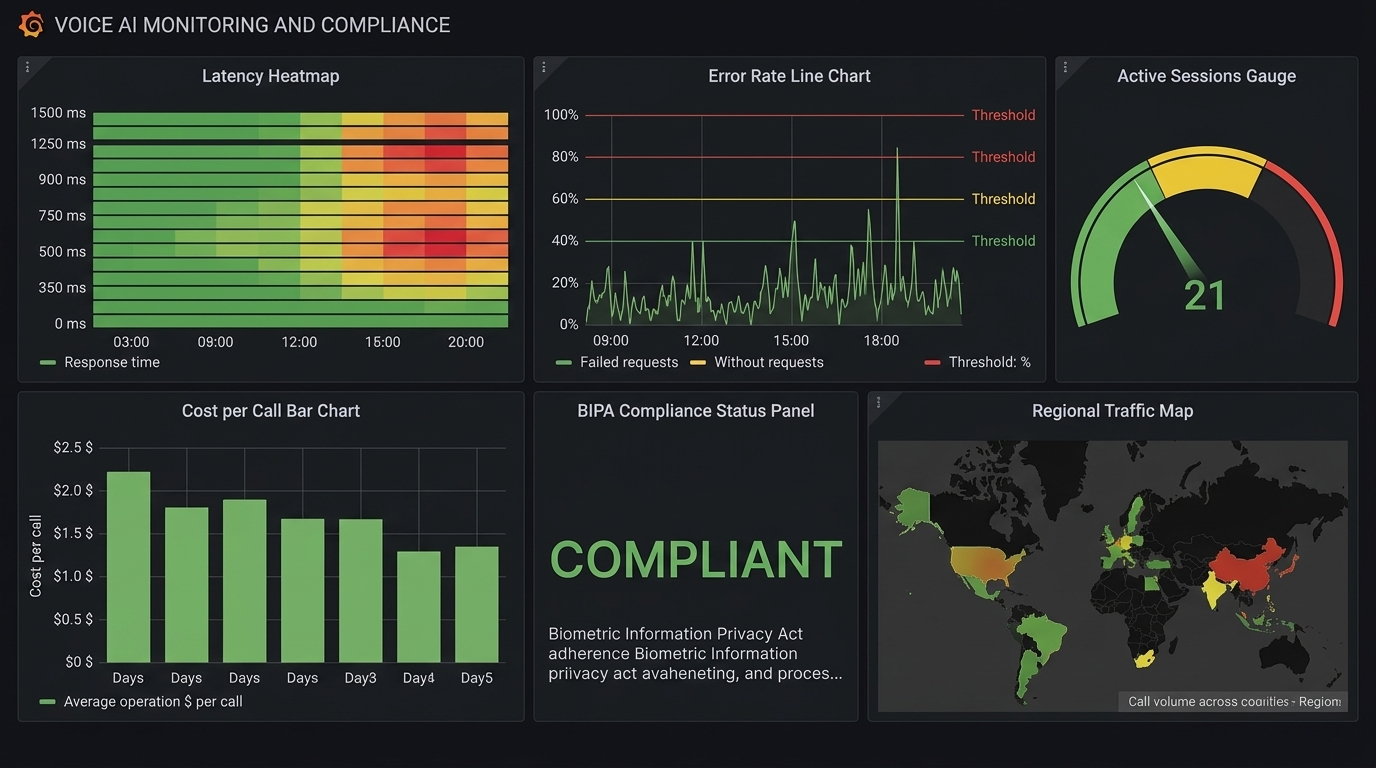
Hero Image: Production dashboard with voice AI metrics, latency graphs, and cost charts

Your voice agent works perfectly in the demo. One user, low latency, great responses. Then you ship it. A hundred users connect simultaneously, latency triples, the TTS queue backs up, and your monthly bill hits five figures.

Production voice AI is fundamentally an infrastructure problem. The AI part -- choosing models, writing prompts, tuning responses -- is the easy part. The hard part is keeping everything fast, reliable, and affordable at scale. The industry median response time is 1.4-1.7 seconds, and 10% of production calls exceed 3-5 seconds. The companies that win are the ones who engineer their way below the 300ms threshold that humans expect from natural conversation.

This guide covers the operational realities of running voice agents in production: infrastructure sizing, the three metrics that actually matter, cost modeling with real numbers, compliance requirements that most teams discover too late, and the operational runbooks that keep systems alive at scale.


Infrastructure Sizing

Voice agents are uniquely resource-intensive. Unlike text chatbots where a single server can handle thousands of concurrent conversations, voice agents consume real-time compute for every active call -- audio processing, model inference, and media routing all happen simultaneously and continuously.

Compute Requirements per Concurrent Call

Each active voice call requires:

Resource API-Based Pipeline Self-Hosted Pipeline
STT processing 1 API call per utterance ~0.3 vCPU (streaming Whisper)
LLM inference 1 API call per turn 1-4 vCPU (small models) or GPU (large)
TTS synthesis 1 API call per response ~0.5 vCPU (Kokoro) or GPU (ElevenLabs-quality)
Audio routing ~0.1 vCPU ~0.1 vCPU
Memory 200-500MB per session 200-500MB per session
Network ~64kbps per direction ~64kbps per direction

Scaling Targets

Concurrent Calls API-Based Infrastructure Self-Hosted Infrastructure
10 Standard web server (4 vCPU) 1x 8-vCPU server + 1x T4 GPU
100 2x web servers behind load balancer 4x 8-vCPU servers + 2x A10 GPUs
1,000 4x web servers, connection pooling Auto-scaling group + 8x A10 GPUs
10,000 Dedicated API tier, rate limit management Kubernetes cluster + GPU pool

The GPU Utilization Insight

GPU utilization for TTS (and self-hosted STT) is bursty. Calls don't generate speech continuously -- there are pauses, listening periods, and processing gaps. A well-designed batching system can achieve 70-80% GPU utilization by queuing TTS requests across concurrent calls.

import asyncio
from collections import deque

class TTSBatchQueue:
    """Batch TTS requests across concurrent calls for better GPU utilization.

    Instead of processing one TTS request at a time, collect requests
    and process them in batches. This increases throughput by 3-5x.
    """

    def __init__(self, model, batch_size: int = 8, max_wait_ms: float = 50):
        self.model = model
        self.batch_size = batch_size
        self.max_wait_ms = max_wait_ms
        self.queue: deque = deque()
        self.processing = False

    async def enqueue(self, text: str, voice: str) -> bytes:
        """Add a TTS request to the batch queue."""
        future = asyncio.get_event_loop().create_future()
        self.queue.append({"text": text, "voice": voice, "future": future})

        if not self.processing:
            asyncio.create_task(self._process_batch())

        return await future

    async def _process_batch(self):
        """Process queued requests in batches."""
        self.processing = True

        while self.queue:
            # Wait briefly to accumulate more requests
            await asyncio.sleep(self.max_wait_ms / 1000)

            # Collect up to batch_size requests
            batch = []
            while self.queue and len(batch) < self.batch_size:
                batch.append(self.queue.popleft())

            # Process batch on GPU
            texts = [r["text"] for r in batch]
            voices = [r["voice"] for r in batch]
            results = await self.model.batch_synthesize(texts, voices)

            # Return results to callers
            for request, audio in zip(batch, results):
                request["future"].set_result(audio)

        self.processing = False
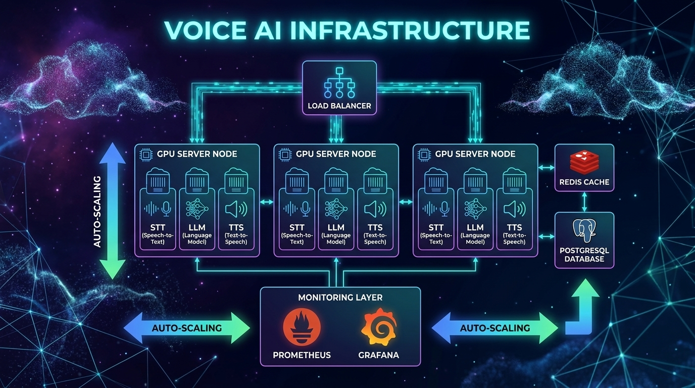
Architecture Diagram: Production voice AI infrastructure with load balancers and GPU pools

Connection Management

WebRTC connections are stateful and expensive. Each connection maintains DTLS encryption context, SRTP session keys, ICE candidate state, and codec negotiation state.

Plan for ~100 concurrent WebRTC connections per media server instance. Beyond that, you need a distributed architecture with a signaling layer that routes connections to available media servers.

For telephony (SIP/PSTN), each trunk supports a fixed number of concurrent calls. Plan capacity with your telephony provider (Twilio, Vonage) and implement graceful rejection when capacity is reached.


The Three Metrics That Matter

Voice AI monitoring requires fundamentally different metrics than traditional web services. Response time and error rate aren't enough. You need voice-specific observability.

graph TD subgraph Metric 1: TTFB A1[User finishes speaking] --> A2[Timer starts] A2 --> A3[STT finalization] A3 --> A4[LLM inference] A4 --> A5[TTS generation] A5 --> A6[First audio byte reaches user] A6 --> A7[Timer stops] A7 --> A8{P95 < 500ms?} A8 -->|Yes| A9[Healthy] A8 -->|No| A10[Alert: Scale TTS/LLM] end style A1 fill:#4CAF50,color:#fff style A9 fill:#4CAF50,color:#fff style A10 fill:#f44336,color:#fff

1. Time-to-First-Byte (TTFB)

This is the interval between the user finishing their utterance and the first audio byte of the response reaching their speaker. It's the single most important metric for user experience.

Threshold Impact Action
< 300ms Feels like natural conversation Gold standard
300-500ms Users notice slight delay but tolerate Target for production
500-800ms Noticeable lag, users start talking over AI Needs optimization
> 800ms Users hang up or repeat themselves Critical -- page on-call

The 300ms rule: Human conversation has a natural pause of about 300ms between turns. This is neurologically hardwired -- exceeding it triggers stress. The industry median is 1.4-1.7 seconds, which is 5x slower than human expectation.

Production leaders are achieving sub-200ms by combining Cartesia TTS (40ms TTFA), optimized STT streaming, and fast LLMs. Some teams report sub-97ms TTS with Qwen3-TTS-Flash and sub-138ms with ElevenLabs Flash.

Break TTFB into sub-components and alert on each independently:

import time
import logging
from dataclasses import dataclass, field

@dataclass
class TTFBTracker:
    """Track TTFB broken down by pipeline stage.

    Each component reports its latency. Alerts fire when any stage
    exceeds its individual threshold OR when total TTFB exceeds target.
    """
    stt_ms: float = 0
    llm_ms: float = 0
    tts_ms: float = 0
    network_ms: float = 0

    # Thresholds per component
    stt_threshold: float = 200
    llm_threshold: float = 350
    tts_threshold: float = 200
    total_threshold: float = 500

    @property
    def total_ms(self) -> float:
        return self.stt_ms + self.llm_ms + self.tts_ms + self.network_ms

    def check_alerts(self) -> list[str]:
        alerts = []
        if self.stt_ms > self.stt_threshold:
            alerts.append(f"STT latency {self.stt_ms:.0f}ms > {self.stt_threshold}ms")
        if self.llm_ms > self.llm_threshold:
            alerts.append(f"LLM latency {self.llm_ms:.0f}ms > {self.llm_threshold}ms")
        if self.tts_ms > self.tts_threshold:
            alerts.append(f"TTS latency {self.tts_ms:.0f}ms > {self.tts_threshold}ms")
        if self.total_ms > self.total_threshold:
            alerts.append(f"Total TTFB {self.total_ms:.0f}ms > {self.total_threshold}ms")
        return alerts

    def log_metrics(self, call_id: str):
        """Emit structured metrics for dashboarding."""
        logging.info(
            f"TTFB call={call_id} "
            f"stt={self.stt_ms:.0f}ms "
            f"llm={self.llm_ms:.0f}ms "
            f"tts={self.tts_ms:.0f}ms "
            f"net={self.network_ms:.0f}ms "
            f"total={self.total_ms:.0f}ms"
        )

2. Word Error Rate (WER)

How accurately the STT component transcribes user speech. High WER means the LLM receives garbled input and generates irrelevant responses.

WER Quality Impact
< 5% Excellent (near human parity) 1 error per 20-word sentence
5-10% Good, highly usable 1 error per 10-word sentence
10-20% Fair, needs review 2 errors per 10-word sentence
> 20% Poor, needs additional training Unusable for production

WER varies dramatically by segment. A 3% overall WER might hide a 15% WER for non-native speakers or a 25% WER for callers on noisy phone lines. Monitor WER by:

  • Audio quality (clean vs phone vs noisy)
  • Speaker accent (native vs non-native)
  • Domain vocabulary (general vs technical/medical/legal)
  • Audio codec (opus vs G.711 -- phone codecs are lossy)
# Simple WER calculation for production monitoring
def word_error_rate(reference: str, hypothesis: str) -> float:
    """Calculate WER between reference (ground truth) and hypothesis (STT output).

    Uses dynamic programming (Levenshtein distance on word level).
    In production, sample ~1% of calls and have humans verify transcripts.
    """
    ref_words = reference.lower().split()
    hyp_words = hypothesis.lower().split()

    # Dynamic programming matrix
    d = [[0] * (len(hyp_words) + 1) for _ in range(len(ref_words) + 1)]
    for i in range(len(ref_words) + 1):
        d[i][0] = i
    for j in range(len(hyp_words) + 1):
        d[0][j] = j

    for i in range(1, len(ref_words) + 1):
        for j in range(1, len(hyp_words) + 1):
            if ref_words[i-1] == hyp_words[j-1]:
                d[i][j] = d[i-1][j-1]
            else:
                d[i][j] = 1 + min(d[i-1][j], d[i][j-1], d[i-1][j-1])

    return d[len(ref_words)][len(hyp_words)] / max(len(ref_words), 1)

3. Conversation Drop-Off Rate

The percentage of conversations where the user disconnects prematurely -- they didn't get what they needed.

Drop-Off Severity Action
< 10% Healthy Monitor trends
10-20% Warning Investigate UX issues
> 20% Critical System is failing users, escalate

Correlate drop-offs with latency spikes. In most production systems, there's a clear threshold -- when TTFB exceeds 600-800ms, drop-off rate spikes exponentially. Track the correlation:

import numpy as np

def analyze_dropoff_correlation(call_records: list[dict]) -> dict:
    """Analyze relationship between TTFB and drop-off rate.

    Returns the TTFB threshold above which drop-off rate spikes.
    """
    # Group calls by TTFB bucket (100ms increments)
    buckets = {}
    for call in call_records:
        bucket = int(call["avg_ttfb_ms"] / 100) * 100
        if bucket not in buckets:
            buckets[bucket] = {"total": 0, "dropped": 0}
        buckets[bucket]["total"] += 1
        if call["dropped"]:
            buckets[bucket]["dropped"] += 1

    # Calculate drop-off rate per bucket
    rates = {}
    for bucket, counts in sorted(buckets.items()):
        rate = counts["dropped"] / max(counts["total"], 1)
        rates[bucket] = rate

    # Find the inflection point (where drop-off rate > 2x baseline)
    baseline = rates.get(300, rates.get(400, 0.05))
    threshold = None
    for bucket, rate in sorted(rates.items()):
        if rate > baseline * 2 and threshold is None:
            threshold = bucket

    return {
        "rates_by_bucket": rates,
        "inflection_threshold_ms": threshold,
        "baseline_dropoff": baseline
    }

Cost Modeling: APIs vs Self-Hosted

The cost difference between API-based and self-hosted voice AI is staggering at scale. Understanding the trade-offs is critical for budgeting.

API-Based Costs (Per Minute of Conversation)

Component Budget Option Mid-Tier Premium
STT GPT-4o Mini Transcribe $0.003 Deepgram Nova-3 $0.0077 Google Chirp Enhanced $0.036
LLM GPT-4o-mini ~$0.005 GPT-4o ~$0.02 Claude Opus ~$0.05
TTS OpenAI tts-1 ~$0.015 ElevenLabs Flash ~$0.07 ElevenLabs v3 ~$0.10
Telephony Twilio ~$0.015 Twilio ~$0.015 Twilio ~$0.015
Total ~$0.04/min ~$0.11/min ~$0.20/min

At Scale: 100,000 Minutes/Month

Architecture Monthly Cost Notes
Budget API pipeline $4,000 GPT-4o-mini + OpenAI TTS
Standard API pipeline $11,000 GPT-4o + Deepgram + ElevenLabs
OpenAI Realtime API $30,000 All-in-one end-to-end
Bland AI (managed) $9,000 $0.09/min, everything included
Retell AI (managed) $5,000-15,000 Volume discounts at enterprise
Self-hosted (full stack) $10,000 Fixed infrastructure cost

The Self-Hosted Break-Even

Self-hosted infrastructure (faster-whisper + Llama 70B quantized + Kokoro TTS):

Infrastructure Monthly Cost Capacity
2x A10 GPU (STT) ~$2,400 ~500K min/month
4x A10 GPU (LLM) ~$4,800 ~500K min/month
1x A10 GPU (TTS) ~$1,200 ~500K min/month
4x 16-vCPU servers ~$1,600 Networking + routing
Total ~$10,000/month ~500K min/month

That's $0.02/minute -- 5-15x cheaper than API-based approaches. But you need an engineering team (2-3 people) to maintain it. The break-even including engineering cost is approximately 100,000-150,000 minutes/month.

The Hybrid Strategy

The smartest approach combines both:

class CostOptimizedRouter:
    """Route to self-hosted or API based on current load and cost efficiency.

    Self-host the expensive components (TTS at scale).
    Use APIs for components where reliability matters most (STT for streaming).
    """

    def __init__(self):
        self.self_hosted_tts_capacity = 100  # concurrent requests
        self.current_tts_load = 0

    def get_tts_provider(self) -> str:
        # If self-hosted has capacity, use it ($0.001/min)
        if self.current_tts_load < self.self_hosted_tts_capacity * 0.8:
            return "kokoro_self_hosted"
        # Overflow to API ($0.07/min) -- still cheaper than dropping calls
        return "elevenlabs_api"

    def get_stt_provider(self) -> str:
        # Always use API for STT -- reliability matters most for first stage
        return "deepgram_api"

    def get_llm_provider(self, complexity: str) -> str:
        if complexity == "simple":
            return "gpt-4o-mini"   # $0.005/min
        elif complexity == "complex":
            return "gpt-4o"        # $0.02/min
        else:
            return "claude-sonnet"  # $0.01/min
graph LR A[Incoming Call] --> B{Load Check} B -->|Under 80% capacity| C[Self-Hosted TTS
$0.001/min] B -->|Over 80% capacity| D[API TTS Overflow
$0.07/min] C --> E[Audio Out] D --> E F[STT] -->|Always API| G[Deepgram Nova-3
Reliability priority] H{Query Complexity} -->|Simple| I[GPT-4o-mini
$0.005/min] H -->|Complex| J[GPT-4o
$0.02/min] style C fill:#4CAF50,color:#fff style D fill:#FF9800,color:#fff style I fill:#4CAF50,color:#fff style J fill:#2196F3,color:#fff

Compliance: The Requirements Most Teams Discover Too Late

Voice AI introduces compliance requirements that text-based systems don't have. Voice data is biometric data under many privacy frameworks, and enforcement is getting serious.

BIPA (Illinois Biometric Information Privacy Act)

BIPA applies when your voice AI extracts voiceprints (speaker embeddings, diarization, speaker profiles).

Requirements:
- Written notice of purpose and duration BEFORE collection
- Written release/consent from each individual
- Publicly posted retention and destruction schedule
- Retention limit: no longer than 3 years (or when initial purpose is satisfied)
- Security: robust encryption, access controls, "reasonable standard of care"

Penalties:
- $1,000 per negligent violation
- $5,000 per reckless or intentional violation
- Per person, per incident

Enforcement is real: In December 2025, Fireflies.AI Corp was hit with a class action for BIPA violations with their AI meeting assistant. The DOJ also issued a December 2024 rule restricting transactions involving Americans' bulk biometric data, with a broad definition that includes voice prints.

GDPR (EU/EEA)

Under GDPR, voice recordings are always personal data. Biometric voiceprints are special category data (Article 9), requiring the highest level of protection.

Requirements:
- Explicit consent (not legitimate interest, not contractual necessity)
- Consent must be: freely given, specific, informed, unambiguous
- Silence or pre-ticked boxes do NOT qualify as consent
- Must disclose: what data collected, why, how used, how long stored
- Right to deletion -- users can request all voice data be destroyed

Penalties: Up to 4% of annual global turnover or 20 million EUR (whichever is greater)

EU AI Act (effective August 2, 2026):
- Limited risk (most customer service agents): Must inform users they're talking to AI
- High risk (hiring, credit, legal agents): Detailed documentation, conformity assessment required
- Transparency obligations are mandatory -- no opt-out

US State Laws Expanding

  • Texas CUBI Act: Similar to BIPA, covers biometric data
  • Washington State: Biometric identifier protections
  • California CCPA/CPRA: Voice data as personal information, right to deletion
  • TCPA: Applies to outbound AI calling -- consent requirements for automated calls

Implementation Checklist

class ComplianceManager:
    """Ensure voice AI pipeline meets compliance requirements.

    Call check_compliance() before starting any voice session.
    """

    def __init__(self):
        self.consent_store = {}  # user_id -> consent record
        self.retention_days = 90  # Max retention period

    def check_compliance(self, user_id: str, user_state: str) -> dict:
        """Pre-call compliance checks."""
        issues = []

        # 1. AI disclosure -- ALWAYS required
        must_disclose_ai = True

        # 2. Consent check
        consent = self.consent_store.get(user_id)
        if not consent:
            issues.append("No consent on file -- must obtain before processing")
        elif consent.get("expired"):
            issues.append("Consent expired -- must re-obtain")

        # 3. BIPA check (Illinois callers)
        if user_state == "IL":
            if not consent or not consent.get("bipa_written_release"):
                issues.append("BIPA: Written release required for Illinois callers")

        # 4. Recording consent (two-party consent states)
        two_party_states = ["CA", "CT", "FL", "IL", "MD", "MA", "MT",
                           "NH", "PA", "WA"]
        if user_state in two_party_states:
            if not consent or not consent.get("recording_consent"):
                issues.append(f"Two-party consent required in {user_state}")

        # 5. GDPR (EU callers)
        eu_countries = ["DE", "FR", "IT", "ES", "NL", "BE", "AT", "SE",
                       "PL", "DK", "FI", "IE", "PT", "CZ", "RO", "HU"]
        if user_state in eu_countries:
            if not consent or not consent.get("gdpr_explicit"):
                issues.append("GDPR: Explicit consent required for EU callers")

        return {
            "compliant": len(issues) == 0,
            "issues": issues,
            "must_disclose_ai": must_disclose_ai,
            "disclosure_text": (
                "This call is being handled by an AI assistant "
                "and may be recorded for quality purposes."
            )
        }

    def schedule_data_deletion(self, user_id: str):
        """Schedule voice data deletion per retention policy."""
        # In production: use a task queue (Celery, Cloud Tasks)
        # to delete recordings after retention_days
        pass

Operational Runbook

Scaling Triggers

Metric Threshold Action
TTFB P95 > 400ms Scale up TTS instances
GPU utilization > 75% sustained (5 min) Add GPU capacity
Connection count > 80% of limit Scale media servers
Error rate > 1% Page on-call, investigate
Drop-off rate > 15% Emergency -- investigate latency/quality
API rate limit hits Any Implement backoff, upgrade plan

Common Failure Modes and Fixes

1. TTS Queue Saturation
- Symptom: Response latency increases linearly with concurrent calls
- Cause: Too many concurrent synthesis requests for available GPU/API capacity
- Fix: Increase TTS replicas, implement request prioritization, add API overflow

2. STT Timeout on Long Utterances
- Symptom: Transcription fails or returns empty for users speaking 30+ seconds
- Cause: Whisper's 30-second chunk boundary, or API timeout
- Fix: Implement chunked streaming with partial results, increase timeout

3. LLM Cold Start
- Symptom: First request after scaling takes 5-10 seconds
- Cause: Model loading into GPU memory, JIT compilation
- Fix: Keep warm instances, implement health checks that load models on startup

4. WebRTC ICE Failure
- Symptom: Some users can't connect, especially on corporate networks
- Cause: NAT traversal fails for restrictive firewalls
- Fix: Ensure TURN server availability, monitor ICE candidate types, offer WebSocket fallback

5. Echo Loop
- Symptom: Agent hears its own output and responds to itself in a loop
- Cause: Acoustic echo cancellation (AEC) not working, speaker audio leaking into microphone
- Fix: Enable WebRTC AEC, reduce speaker volume, add echo detection to pipeline

6. Token Overflow on Long Calls
- Symptom: LLM starts hallucinating or ignoring context after 20+ minute call
- Cause: Conversation context exceeds LLM context window
- Fix: Implement conversation summarization, trim old messages, track token count

Incident Response Template

## Voice AI Incident Report

**Severity**: P1/P2/P3
**Duration**: Start -> End (total minutes)
**Impact**: X% of calls affected, Y calls dropped

### Timeline
- HH:MM - Alert triggered: [metric] exceeded [threshold]
- HH:MM - On-call acknowledged
- HH:MM - Root cause identified: [description]
- HH:MM - Mitigation applied: [action taken]
- HH:MM - Metrics returned to normal

### Root Cause
[Technical description of what failed and why]

### Metrics During Incident
- TTFB P95: XXms -> XXms (normal: XXms)
- Drop-off rate: XX% -> XX% (normal: XX%)
- Error rate: XX% -> XX% (normal: XX%)

### Action Items
- [ ] Short-term fix: [description]
- [ ] Long-term fix: [description]
- [ ] Monitoring improvement: [new alert or dashboard]

The End-to-End Latency Budget

Here's how to allocate your latency budget across the pipeline to hit the 800ms P95 target (the threshold before drop-off rates spike):

Total Budget: 800ms P95
==============================================
Network edge hop:           40ms   ( 5%)
Audio buffering + decoding: 55ms   ( 7%)
STT (streaming):           200ms   (25%)  <- Use Deepgram with 300ms endpointing
LLM inference:             350ms   (44%)  <- Biggest component, use GPT-4o-mini
TTS:                       105ms   (13%)  <- Use Cartesia (40ms) or ElevenLabs Flash (75ms)
Service hops:               50ms   ( 6%)  <- Connection pooling, colocated services
==============================================
Total:                     800ms   (100%)

Optimization Strategies by Stage

Stage Current Optimization After
STT 300ms Switch from batch to streaming, reduce endpointing 150ms
LLM 500ms GPT-4o -> GPT-4o-mini, shorter system prompt 250ms
TTS 250ms OpenAI TTS -> Cartesia Sonic (40ms) 90ms
Network 100ms Colocate services, connection pooling 40ms
Total 1,150ms 530ms

Streaming optimization can save an additional 300-600ms by overlapping stages:
- Start LLM while STT is finalizing
- Start TTS on the first LLM sentence (don't wait for full response)
- Start audio playback on the first TTS chunk


Monitoring Dashboard

Every production voice AI system needs these dashboards:

Real-Time Dashboard (refreshes every 10s)

  • Active concurrent calls (with capacity utilization %)
  • TTFB P50/P95/P99 (last 5 minutes)
  • Error rate (last 5 minutes)
  • GPU utilization per instance

Hourly Dashboard

  • Call volume by hour (with day-over-day comparison)
  • TTFB distribution histogram
  • WER by audio quality segment
  • Drop-off rate trend
  • Cost per minute trend

Daily Dashboard

  • Total calls, total minutes, total cost
  • WER broken down by accent/language/audio quality
  • Top 10 function calling errors
  • Compliance audit: consent rate, disclosure delivered rate
  • Cost breakdown by component (STT/LLM/TTS/telephony)
Comparison Visual: Production monitoring dashboard layout

The Bottom Line

Production voice AI is a systems engineering challenge. The AI models are good enough. The frameworks are mature. What separates successful deployments from failed ones is the operational foundation:

  1. Size infrastructure for peaks, not averages. Voice traffic is bursty -- Monday morning call volume can be 5x Sunday afternoon.

  2. Monitor the right metrics: TTFB, WER, and drop-off rate. Not just CPU and memory. A system with perfect uptime but 2-second TTFB is failing its users.

  3. Model your costs before you scale. The difference between TTS providers can be 10-100x. Self-hosting saves 5-15x above 100K minutes/month.

  4. Handle compliance early. Retrofitting consent and privacy controls is expensive and legally risky. BIPA penalties are $1,000-$5,000 per incident. The EU AI Act is mandatory starting August 2026.

  5. Build for hybrid. Self-host the expensive components (TTS), use APIs for the critical ones (STT), and overflow to APIs when self-hosted capacity is exhausted.

  6. Hit the 300ms target or get as close as possible. Every millisecond above 300ms increases drop-off. The industry median is 1.4 seconds -- beating that is your competitive advantage.

Voice AI is moving from novelty to infrastructure. The teams that treat it as an infrastructure problem -- not just an AI problem -- will build the products that win.

Sources & References:
1. Twilio — "Voice API Documentation" — https://www.twilio.com/docs/voice
2. EU AI Act — "Regulation (EU) 2024/1689" — https://eur-lex.europa.eu/eli/reg/2024/1689/oj
3. Daily.co — "Real-Time Voice Infrastructure" — https://www.daily.co/


This is the final post in the AmtocSoft Voice AI series. We've covered TTS engines, STT models, building voice agents with Pipecat, architecture decisions, and now production operations. The full series gives you everything you need to go from zero to a production voice agent.

About the Author

Toc Am

Founder of AmtocSoft. Writing practical deep-dives on AI engineering, cloud architecture, and developer tooling. Previously built backend systems at scale. Reviews every post published under this byline.

LinkedIn X / Twitter

Published: 2026-04-06 · Written with AI assistance, reviewed by Toc Am.

Get These In Your Inbox

Weekly deep-dives on AI engineering, no fluff. Join the newsletter →

Subscribe (free)

Or grab the book ($39, ~100 pages) · Buy me a coffee

Buy Me a Coffee · 🔔 YouTube · 💼 LinkedIn · 🐦 X/Twitter
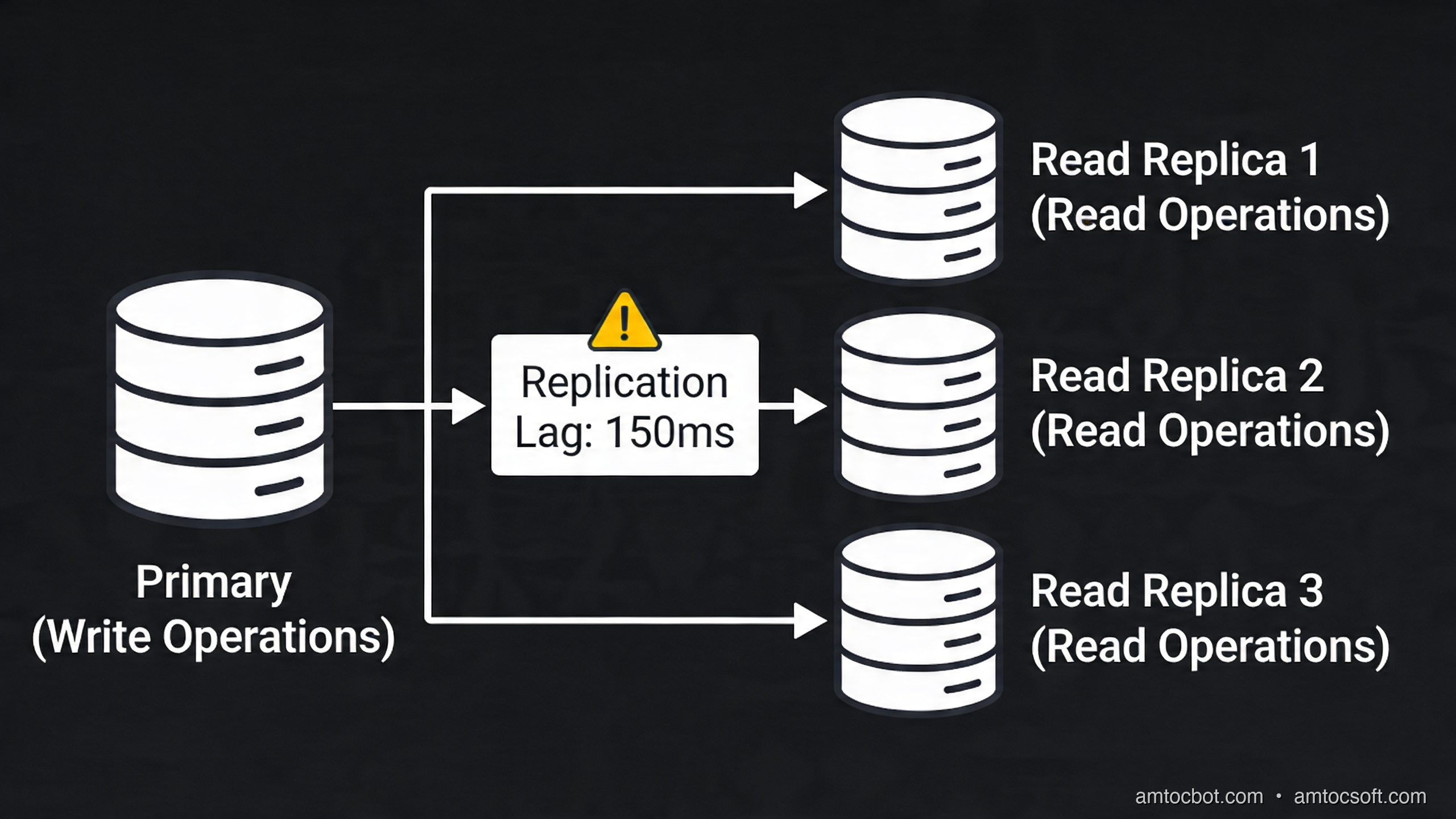
Attention Is All You Need, Explained Simply

We published a plain-language walkthrough of the 2017 transformer paper — queries, keys, values, multi-head attention, and why no-recurrence...