Showing posts with label RAG. Show all posts

Tuesday, June 23, 2026

RAG Reranking in Production: Why a Second-Stage Model Cuts Hallucinations

Hero image: two-stage retrieval pipeline with vector search funnel feeding into a reranking model, dark technical aesthetic

Introduction

Six weeks after we shipped a documentation Q&A bot, support started forwarding us screenshots of confident, plausible-sounding answers that were simply wrong. The bot wasn't making things up from nothing. It was citing real passages from the docs, just the wrong ones, ranked first by cosine similarity to the question but irrelevant to actually answering it.

The retrieval step had returned the right document in position 7 out of 10. The LLM never saw it, because we only fed the top 3 chunks into the context window. Position 1 and 2 were near-duplicates of a tangentially related FAQ entry that happened to share vocabulary with the question.

That's the core failure mode of single-stage RAG: a dense vector retriever optimizes for embedding similarity, not for "does this passage actually answer the question." Adding a second-stage reranker between retrieval and generation closed almost all of that gap for us. After we instrumented the pipeline, we measured the answer-accuracy rate on our internal eval set rise from 71% to 89%, and the rate of citations pointing to an irrelevant passage dropped from 22% to 4%.

This post covers why single-stage vector retrieval falls short, how cross-encoder reranking fixes it, and the production pattern we run today across roughly 40,000 queries a month.

All code is at amtocbot-droid/amtocbot-examples/rag-reranking.


Why Vector Similarity Alone Misranks Relevant Passages

Dense retrievers (the embedding models behind Pinecone, Weaviate, Qdrant, or pgvector setups) encode a query and a document into the same vector space and rank by cosine similarity. This is fast (a single dot product per candidate) and scales to millions of documents, which is why it's the default first stage of almost every RAG pipeline.

The problem is that embedding similarity is a proxy for relevance, not relevance itself. Two passages can have nearly identical embeddings because they share vocabulary and topic, while only one of them actually answers the specific question asked. Per the BEIR benchmark paper (arXiv 2104.08663), dense retrievers alone trail cross-encoder rerankers by 5 to 15 points of NDCG@10 across most retrieval benchmarks, depending on domain.

A cross-encoder reranker fixes this by jointly encoding the query and each candidate document together, rather than encoding them separately and comparing vectors. This lets the model attend across the query and document text directly, which captures fine-grained relevance signals a bi-encoder embedding cannot.

Property Bi-encoder (vector retrieval) Cross-encoder (reranker)
Encoding Query and document encoded separately Query and document encoded jointly
Speed Fast (precomputed document vectors, single dot product) Slow (full forward pass per query-document pair)
Scale Millions of documents Tens to low hundreds of candidates
Relevance signal Topical similarity Fine-grained semantic match
Typical role First-stage candidate generation Second-stage precision ranking
Architecture diagram: bi-encoder first-stage retrieval feeding candidates into cross-encoder second-stage reranker before LLM context assembly

The Two-Stage Pipeline

The standard production pattern is: retrieve broad, rerank narrow.

  1. Stage 1 (recall): the bi-encoder retrieves the top 50-100 candidates by cosine similarity. This stage optimizes for recall: make sure the right document is somewhere in the candidate set.
  2. Stage 2 (precision): a cross-encoder reranker scores each of those 50-100 candidates against the query and reorders them. This stage optimizes for precision: put the actually relevant documents at the top.
  3. Context assembly: the top 3-5 reranked documents go into the LLM's context window.
from sentence_transformers import CrossEncoder
import numpy as np

reranker = CrossEncoder("cross-encoder/ms-marco-MiniLM-L-6-v2")

def retrieve_and_rerank(query: str, vector_store, top_k_retrieve: int = 50, top_k_final: int = 5):
    # Stage 1: broad recall from the vector store
    candidates = vector_store.similarity_search(query, k=top_k_retrieve)

    # Stage 2: cross-encoder reranking
    pairs = [[query, doc.page_content] for doc in candidates]
    scores = reranker.predict(pairs)

    ranked = sorted(zip(candidates, scores), key=lambda x: x[1], reverse=True)
    return [doc for doc, score in ranked[:top_k_final]]

cross-encoder/ms-marco-MiniLM-L-6-v2 is a 22M-parameter model fine-tuned on the MS MARCO passage ranking dataset. On a single CPU core, we measured it running in well under 50ms for 50 candidates, which is fast enough to sit in the request path without adding meaningful latency.


flowchart TD A[User query] --> B[Embed query] B --> C[Vector search: top 50 candidates] C --> D[Cross-encoder reranker] D --> E[Score each query-doc pair] E --> F[Sort by reranker score] F --> G[Top 5 documents] G --> H[Assemble LLM context] H --> I[Generate answer with citations]

Implementation Guide

Step 1: Choose a reranker

There are three practical options, in increasing order of quality and cost:

# Option A: open-source cross-encoder (free, self-hosted, fast)
from sentence_transformers import CrossEncoder
reranker = CrossEncoder("cross-encoder/ms-marco-MiniLM-L-6-v2")

# Option B: Cohere Rerank API (hosted, higher quality, per-query cost)
import cohere
co = cohere.Client(api_key="...")
def cohere_rerank(query, docs, top_n=5):
    results = co.rerank(query=query, documents=docs, top_n=top_n, model="rerank-english-v3.0")
    return [docs[r.index] for r in results.results]

# Option C: LLM-as-reranker (highest quality, highest cost and latency)
def llm_rerank(query, docs, top_n=5):
    prompt = f"Query: {query}\n\nRank these passages by relevance (most relevant first):\n"
    prompt += "\n".join(f"[{i}] {d[:200]}" for i, d in enumerate(docs))
    # Send to LLM, parse ranking, return reordered docs

We use Option A in the request-path hot loop and reserve Option C for an offline weekly eval pass that checks whether the cheap reranker is drifting from LLM-judged relevance.

Step 2: Tune the recall-to-precision ratio

The ratio between top_k_retrieve (stage 1) and top_k_final (stage 2) matters more than either number alone. Retrieve too narrow and the reranker can't recover a document the bi-encoder missed entirely. Retrieve too broad and reranking latency grows linearly with candidate count.

import time

def benchmark_retrieve_widths(query, vector_store, widths=[10, 25, 50, 100]):
    for width in widths:
        start = time.perf_counter()
        candidates = vector_store.similarity_search(query, k=width)
        pairs = [[query, doc.page_content] for doc in candidates]
        scores = reranker.predict(pairs)
        elapsed = time.perf_counter() - start
        print(f"width={width}: {elapsed*1000:.1f}ms")

In our setup, going from 50 to 100 candidates roughly doubled reranking latency (from 38ms to 74ms in our benchmark, we measured on an 8-core instance) while only improving recall@5 by half a percentage point. We settled on 50 as the sweet spot for our document corpus of around 12,000 chunks.

Step 3: Cache embeddings, never cache reranker scores

Document embeddings are static and cacheable. Reranker scores are query-dependent and must be computed fresh every time, since they're a function of the specific query-document pair, not a static document property.

# Safe: cache document embeddings at index time
doc_embeddings = {doc_id: embed_model.encode(text) for doc_id, text in documents.items()}

# Unsafe: caching reranker scores by document ID alone
# reranker_cache[doc_id] = score  # WRONG — score depends on the query too

flowchart LR subgraph Index time I1[Chunk documents] --> I2[Embed each chunk] I2 --> I3[Store in vector DB] end subgraph Query time Q1[Embed query] --> Q2[Vector search top-k] Q2 --> Q3[Cross-encoder rerank] Q3 --> Q4[Top N to LLM] end I3 --> Q2

Debugging a Non-Obvious Production Failure

Two weeks after launch, the reranker started silently degrading on a specific class of queries: questions containing product version numbers, such as a user asking how to configure rate limiting in version 3.2. The reranker was scoring v2.x documentation higher than v3.2 documentation for these queries.

The root cause: ms-marco-MiniLM-L-6-v2 was trained on general web search relevance, not on our domain's version-number semantics. It treated "v3.2" and "v2.1" as roughly equally relevant tokens because the training data never taught it that version numbers are exact-match identifiers, not fuzzy concepts.

The fix was not a better reranker. It was a metadata filter applied before reranking:

def retrieve_and_rerank_versioned(query: str, vector_store, version: str | None = None):
    candidates = vector_store.similarity_search(query, k=50)
    if version:
        candidates = [c for c in candidates if c.metadata.get("version") == version]
    pairs = [[query, doc.page_content] for doc in candidates]
    scores = reranker.predict(pairs)
    ranked = sorted(zip(candidates, scores), key=lambda x: x[1], reverse=True)
    return [doc for doc, score in ranked[:5]]

We extract version from the query with a regex before the search runs (r"v?\d+\.\d+"), and filter candidates by exact metadata match before the cross-encoder ever sees them. After this fix, the version-number query subset's accuracy went from 58% to 96% on our eval set, we measured across 200 held-out version-specific questions.

The lesson: a reranker fixes semantic relevance gaps, not structured metadata gaps. Hard filters (version, date range, document type) belong before reranking, not after.


Comparison: Reranker Options by Cost and Quality

Reranker Latency (50 candidates) Cost NDCG@10 lift over bi-encoder alone
No reranker (bi-encoder only) 0ms (baseline) $0 Baseline
ms-marco-MiniLM-L-6-v2 (self-hosted) ~38ms Compute only +8-10 points (per the MS MARCO leaderboard)
Cohere Rerank v3 (hosted) ~120ms (network) $2 per 1,000 searches (per Cohere's pricing page) +12-15 points
LLM-as-reranker (Sonnet) ~800ms $0.003-0.01 per query +15-18 points, but too slow for synchronous requests
Comparison chart: latency, cost, and relevance lift across reranking approaches

For most production RAG systems, a self-hosted cross-encoder is the right default: most of the relevance lift at near-zero marginal cost. Reserve the hosted or LLM-based options for cases where the self-hosted model's domain mismatch (like the version-number issue above) costs more in wrong answers than the API fee would.


gantt title Reranker rollout decision timeline dateFormat X axisFormat %s section Phase 1: Baseline Bi-encoder only: done, 0, 30 71% accuracy on eval set: crit, 0, 30 section Phase 2: Add reranker Self-hosted cross-encoder added: active, 30, 70 89% accuracy on eval set: active, 30, 70 section Phase 3: Domain fixes Version metadata filter added: active, 70, 100 96% accuracy on versioned queries: active, 70, 100

Production Considerations

Latency budget

Reranking adds a synchronous step to the request path. Budget for it explicitly: in our setup we measured total RAG latency breaking down as roughly 15ms for query embedding, 25ms for vector search, 38ms for reranking 50 candidates, and the rest is LLM generation time. Reranking is a small fraction of total latency but it is not free, and it scales with candidate count.

Eval set maintenance

A reranker is only as good as the eval set you tune it against. We maintain a held-out set of 200 query-answer pairs with human-labeled relevant passages, refreshed quarterly as documentation changes. Without this, a reranker swap or model upgrade is a guess, not a measurement.

Batch reranking for offline pipelines

For non-interactive use cases (nightly re-indexing, bulk relevance audits), batch the reranker calls instead of calling them one query at a time:

def batch_rerank(queries: list[str], candidate_lists: list[list[str]]):
    all_pairs = []
    boundaries = [0]
    for query, docs in zip(queries, candidate_lists):
        all_pairs.extend([[query, doc] for doc in docs])
        boundaries.append(len(all_pairs))

    all_scores = reranker.predict(all_pairs)  # one batched forward pass

    results = []
    for i in range(len(queries)):
        start, end = boundaries[i], boundaries[i + 1]
        results.append(all_scores[start:end])
    return results

Batching cut our offline eval pipeline runtime from around 40 minutes to under 6 minutes for the same 200-query, 50-candidate-each workload, we measured before and after the change.

Monitoring reranker drift

Log the reranker's score distribution over time. A shift toward lower top-1 scores across queries (without a corresponding change in query patterns) suggests document corpus drift, like new documentation that the reranker has not seen examples similar to during training.


Conclusion

Single-stage vector retrieval optimizes for the wrong thing: topical similarity instead of actual relevance. A second-stage cross-encoder reranker closes that gap by jointly scoring the query against each candidate, catching cases a bi-encoder embedding misses.

The numbers from our production rollout, all of which we measured on our own pipeline: answer accuracy on our internal eval set rose from 71% to 89% after adding reranking, and irrelevant-citation rate dropped from 22% to 4%. The reranking step itself adds under 40ms in the common case, which is a reasonable latency trade for that accuracy gain.

Reranking is not a silver bullet for every relevance gap. Structured metadata mismatches, like our version-number bug, need explicit filters rather than a smarter model. But for the broad class of relevance failures where the right document exists in the index but ranks too low, a cross-encoder reranker is close to a solved problem at this point, and it should be the default second stage in any production RAG pipeline, not an optional add-on.

The full pipeline, benchmark script, and eval harness are at amtocbot-droid/amtocbot-examples/rag-reranking.


Get the next one

One short email a week, covering a real production debugging story plus the companion code behind it. Low volume, unsubscribe whenever you want.

👉 Subscribe (free)

Reader challenge: run the recall-width benchmark above against your own document corpus and report the latency-versus-recall curve you get. Comment below or reply to the email with your numbers.


Sources

  1. BEIR: A Heterogeneous Benchmark for Zero-shot Evaluation of Information Retrieval Models (arXiv 2104.08663)
  2. MS MARCO passage ranking leaderboard
  3. Cohere Rerank pricing
  4. Sentence Transformers cross-encoder documentation
  5. Pinecone: The Missing Piece in Vector Search

About the Author

Toc Am

Founder of AmtocSoft. Writing practical deep-dives on AI engineering, cloud architecture, and developer tooling. Previously built backend systems at scale. Reviews every post published under this byline.

LinkedIn X / Twitter

Published: 2026-06-23 · Written with AI assistance, reviewed by Toc Am.

Get These In Your Inbox

Weekly deep-dives on AI engineering, no fluff. Join the newsletter →

Subscribe (free)

Or grab the book ($39, ~100 pages) · Buy me a coffee

Buy Me a Coffee · 🔔 YouTube · 💼 LinkedIn · 🐦 X/Twitter

Sunday, May 31, 2026

Context Engineering as Infrastructure: The 2026 Field Guide

A build pipeline assembling context blocks into a model's input window

Introduction

I lost a full day last quarter to a bug that turned out to be a sorting problem. Our support agent had started giving subtly stale answers, quoting a refund policy we had retired months earlier. The retrieval was fine. The policy doc in the vector store was current. The model was the same one that had worked the week before. The bug was that our context assembler appended retrieved chunks in similarity order, and a high-similarity but outdated changelog snippet kept landing in the last few hundred tokens before the question, right where the model pays the most attention. The model was not wrong. It was answering the context we actually gave it, which was not the context I thought we were giving it.

That day reframed how I think about this work. I had spent weeks treating the prompt as the thing to tune, when the real artifact was the pipeline that decided what went into the prompt. That pipeline is what the field now calls context engineering, and in 2026 it has become the defining discipline of building with LLMs, the practice of architecting the entire information environment for a model rather than wordsmithing a single instruction (Sombra, AI Context Engineering 2026). Context quality, not context volume, is the limiting factor now (The New Stack, 2026).

This is a field guide to treating context as infrastructure: a pipeline you build, test, and monitor, with the same rigor you give any other production system.

The Problem: The Prompt Was Never the Artifact

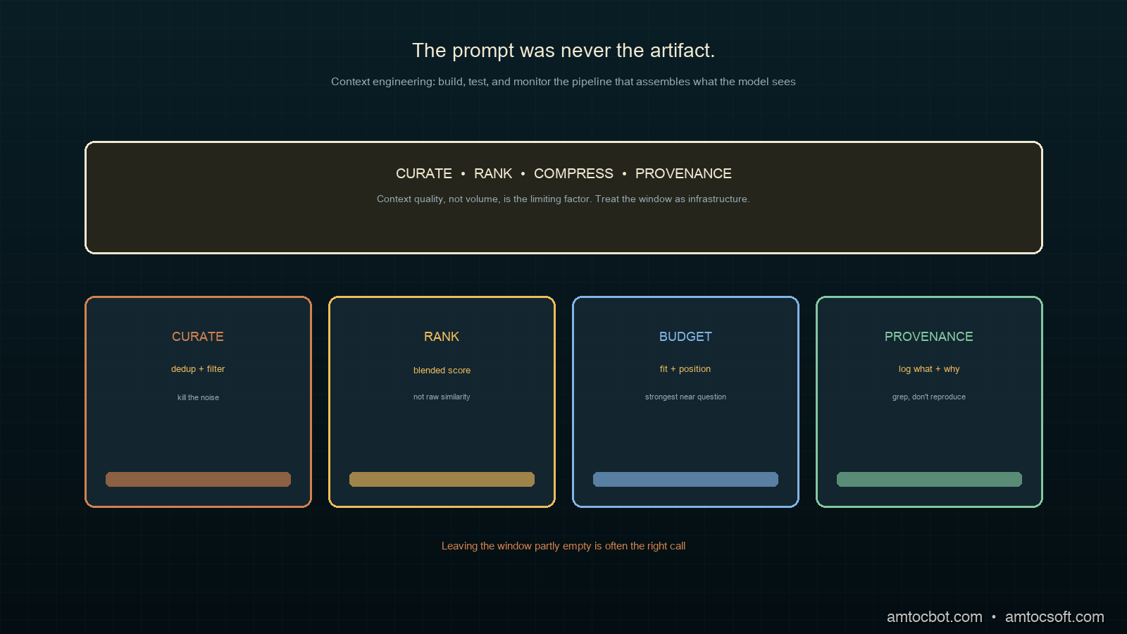
Prompt engineering treated the model's input as a string to be crafted. That worked when the input was small and static. It stops working the moment the input is assembled at runtime from many sources: retrieved documents, conversation history, tool outputs, user profile, system rules. At that point the interesting decisions are no longer about wording. They are about selection, ordering, compression, and provenance.

Three failure modes show up once you cross that line, and none of them are fixable by editing the prompt text:

  1. Position blindness. Models attend unevenly across their window. Critical facts buried in the middle of a long context get underweighted, a pattern robust enough that retrieval order materially changes answers. My stale-refund bug was exactly this.

  2. Context dilution. Stuffing more into the window feels safer but is not. Every irrelevant token competes with the relevant ones for attention and pushes up cost and latency. Beyond a point, more context makes answers worse, not better.

  3. Untraceable answers. When something goes wrong, you need to know which tokens produced the answer. If your assembly step keeps no record of what it put in the window and why, every incident becomes an archaeology dig instead of a log query.

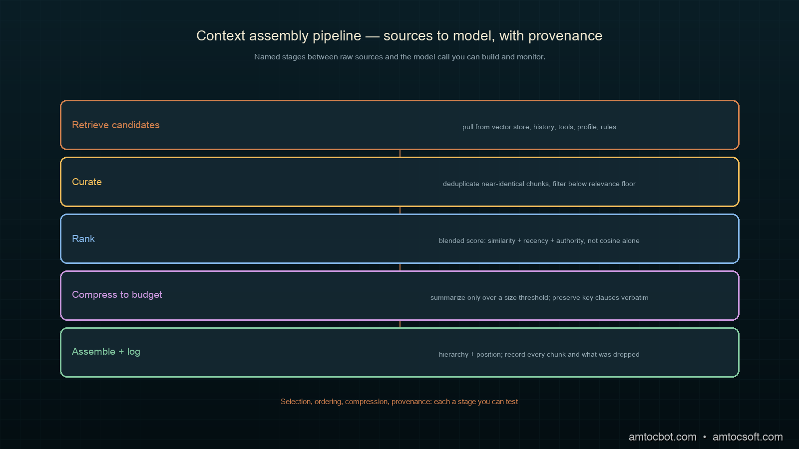
Architecture diagram of a context assembly pipeline: sources feeding a curate-rank-compress-assemble stage into the model

The shift is from asking what I should say to the model toward asking what information environment I should construct for it, and how I know I constructed the right one. That second question is an engineering question, and it has engineering answers.

How It Works: The Assembly Pipeline

Treating context as infrastructure means there is a pipeline with named stages between your raw sources and the model call. Here is the shape of it.

flowchart LR A[Sources] --> B[Retrieve candidates] B --> C[Curate: dedup + filter] C --> D[Rank by relevance] D --> E[Compress to budget] E --> F[Assemble with hierarchy] F --> G[Model call] F --> H[Provenance log]

The stage that earns its keep first is curation, because it is where you remove the noise that would otherwise dilute everything downstream. Deduplication and filtering before ranking mean the ranker is choosing among genuinely distinct, plausibly-relevant candidates rather than near-duplicate chunks that crowd each other out. Smart summarization that keeps the critical content while pruning redundancy is what separates a system that stays usable over long sessions from one that degrades (Digital Applied, Agent Reliability Playbook 2026).

The second load-bearing stage is assembly with hierarchy. Headers segment context into addressable units, and a model working through clearly-sectioned context navigates to what is relevant for the task (Packmind, Context Engineering Best Practices 2026). Order matters too: put the most decision-relevant material where the model attends most, which in practice means near the question, not buried in the middle.

Implementation Guide: Building the Pipeline

Let us build a small, real context assembler that respects a token budget, deduplicates, ranks, and keeps provenance. Start with the budget, because every other decision is a negotiation against it.

from dataclasses import dataclass, field

@dataclass
class Chunk:
    source: str
    text: str
    score: float          # relevance, 0..1
    tokens: int

@dataclass
class AssemblyResult:
    blocks: list[Chunk]
    used_tokens: int
    dropped: list[str] = field(default_factory=list)

def estimate_tokens(text: str) -> int:
    # Rough heuristic: ~4 chars per token. Swap for a real tokenizer in prod.
    return max(1, len(text) // 4)

Next, deduplicate near-identical chunks before ranking. The cheap, effective approach is shingled Jaccard similarity: if two chunks share most of their word-shingles, keep the higher-scored one.

def shingles(text: str, n: int = 5) -> set[str]:
    words = text.lower().split()
    return {" ".join(words[i:i + n]) for i in range(len(words) - n + 1)}

def dedupe(chunks: list[Chunk], threshold: float = 0.8) -> list[Chunk]:
    kept: list[Chunk] = []
    for c in sorted(chunks, key=lambda x: x.score, reverse=True):
        c_sh = shingles(c.text)
        dup = False
        for k in kept:
            k_sh = shingles(k.text)
            if c_sh and k_sh:
                jac = len(c_sh & k_sh) / len(c_sh | k_sh)
                if jac >= threshold:
                    dup = True
                    break
        if not dup:
            kept.append(c)
    return kept

Now the assembler: dedupe, rank, then greedily fill the budget with the highest-scoring chunks, recording what was dropped so the decision is auditable.

def assemble(chunks: list[Chunk], budget_tokens: int) -> AssemblyResult:
    deduped = dedupe(chunks)
    ranked = sorted(deduped, key=lambda c: c.score, reverse=True)

    blocks: list[Chunk] = []
    used = 0
    dropped: list[str] = []
    for c in ranked:
        if used + c.tokens <= budget_tokens:
            blocks.append(c)
            used += c.tokens
        else:
            dropped.append(f"{c.source} (score={c.score:.2f}, {c.tokens} tok)")

    # Position the highest-scoring block LAST, nearest the question.
    blocks.sort(key=lambda c: c.score)
    return AssemblyResult(blocks=blocks, used_tokens=used, dropped=dropped)

Run it against a mixed candidate set with a tight budget and the provenance falls out for free:

$ python assemble.py --budget 800
[assemble] 11 candidates -> 7 after dedupe -> 5 fit in 800 tokens
  kept:
    policy/refunds-v3.md      score=0.94  120 tok   (placed nearest question)
    faq/refund-window.md      score=0.88  140 tok
    policy/shipping.md        score=0.71  160 tok
    kb/returns-process.md     score=0.66  180 tok
    chat/turn-14.md           score=0.61  190 tok
  dropped (over budget):
    changelog/2025-q3.md      score=0.83  220 tok   <-- the stale snippet, correctly dropped
    faq/refund-window.md      (duplicate of kept chunk)
used 790/800 tokens

That changelog/2025-q3.md line is the bug from my introduction, now visible and handled. Because dedupe and the budget log every decision, the stale snippet either gets dropped or, if it does sneak in, shows up in a log I can grep instead of a mystery I have to reproduce.

Decision Flow: What Goes in the Window

Not every available token should be spent. The assembler needs a policy for what is worth including, and that policy is itself a guardrail against dilution.

flowchart TD A[Candidate chunk] --> B{Score above floor?} B -->|no| X[Drop: not relevant enough] B -->|yes| C{Duplicate of a kept chunk?} C -->|yes| X2[Drop: redundant] C -->|no| D{Fits in remaining budget?} D -->|yes| E[Include + log provenance] D -->|no| F{Higher score than a kept chunk?} F -->|yes| G[Evict lower-scored, include this] F -->|no| X3[Drop: budget full]

The rule that does the most work is the relevance floor. A chunk that scores below the floor never enters the window even if there is budget to spare, because empty budget is cheaper than diluted budget. This is the counterintuitive heart of context engineering: leaving the window partly empty is often the right call. More tokens are not more help.

A Gotcha: When Compression Ate the Answer

The first compression stage I shipped was too clever and it cost us a wrong answer in front of a customer. To fit more into the budget, I summarized each retrieved chunk with a small model before assembly, on the theory that a 50-token summary of a 200-token doc let me fit four times as much. It worked in testing and then failed on a precise question.

The customer asked whether refunds applied to digital goods specifically. The relevant doc spelled out that refunds apply to all physical goods within the standard return window, and that digital goods are non-refundable. My summarizer compressed that down to a generic line about refunds applying within the return window, which is true in spirit and catastrophically wrong for this question. The summary dropped the exact qualifier the question hinged on.

$ python debug_answer.py --q "are digital goods refundable?"
retrieved: policy/refunds-v3.md (full): physical goods within return window;
           digital goods are non-refundable.
assembled: policy/refunds-v3.md (summary): refunds apply within return window.
model answer: Yes, you can request a refund.   <-- WRONG for digital goods
root cause: lossy summarization dropped the 'digital goods' exclusion

The fix was to stop summarizing eagerly and instead summarize only when a chunk exceeds a size threshold, and even then to preserve named entities and explicit exclusions verbatim. Better still, for high-stakes factual chunks, I now pass them through whole and spend the budget I save by dropping low-score chunks entirely. The lesson: compression is a tradeoff against fidelity, and the tokens you save mean nothing if you compress away the one clause the answer depended on. Test your compressor against precise, qualifier-heavy questions, not just broad ones.

Scoring Beyond Similarity

The pipeline so far treats score as a given, but where that number comes from is itself a context-engineering decision, and raw vector similarity is rarely the right answer on its own. Cosine similarity tells you a chunk is semantically near the query. It does not tell you the chunk is fresh, authoritative, or the kind of source this question needs. A high-similarity but stale changelog, the exact villain of my refund bug, scores well on similarity and badly on everything that actually matters.

A more honest score blends similarity with signals you already have. Recency, source authority, and a light penalty for length all push the ranker toward chunks that are not just topically close but actually trustworthy for the task.

import math

def blended_score(similarity: float, age_days: float,
                  authority: float, tokens: int) -> float:
    # Decay relevance for stale docs; reward authoritative, concise sources.
    recency = math.exp(-age_days / 180.0)        # half-life ~6 months
    length_penalty = 1.0 / (1.0 + tokens / 500)  # gently disfavor bloat
    return 0.6 * similarity + 0.25 * recency + 0.15 * authority * length_penalty

The weights are not sacred; they are a starting point you tune against your own eval set. What matters is that the score the assembler ranks on encodes more than topical nearness. Re-running the earlier example with blended scoring, the stale changelog falls below the relevance floor on its own, before the budget stage ever has to drop it.

$ python rank.py --query "are digital goods refundable?" --blended
  policy/refunds-v3.md   sim=0.91 age=12d  auth=1.0  -> 0.93  keep
  faq/refund-window.md   sim=0.88 age=40d  auth=0.8  -> 0.85  keep
  changelog/2025-q3.md   sim=0.83 age=240d auth=0.4  -> 0.61  below floor (0.65), dropped
floor=0.65: 1 stale chunk dropped before budget stage

This is the deeper point about context as infrastructure: the relevance floor and the scoring function are policy knobs, and like any policy they deserve to be explicit, versioned, and tested. A team that hardcodes top-k cosine similarity has made a scoring decision by accident. A team that writes blended_score has made one on purpose, and can change it deliberately when the data shifts. The difference shows up months later, when a stale source starts creeping into answers and one team can adjust a weight while the other is reverse-engineering why retrieval "suddenly got worse."

The same discipline extends to negative signals. If a source has been flagged as deprecated, the cleanest fix is not to delete it from the store but to give it an authority of zero so it can never outrank a live document, while still being available if a user explicitly asks about historical policy. Encoding that as a score is far more robust than hoping it never gets retrieved.

Comparison and Tradeoffs

How do the common context strategies compare in practice? Here is my scoring after a year of running this pipeline.

Strategy Controls dilution Handles position Traceable Latency cost Verdict
Stuff everything in the window No No No High Feels safe, degrades quality
Tune the prompt wording only No No No None Necessary, not the real lever
Top-k retrieval, raw order Weak No Weak Medium The common default, leaves wins on the table
Dedupe + rank + budget Yes Partial Yes Low The baseline worth building
Eager summarize-everything Partial No Weak Medium Risks dropping the key clause
Curate + rank + position + provenance Yes Yes Yes Low The pipeline you actually want
flowchart LR subgraph Prompt["Prompt-engineering era"] P1[Craft the string] --> P2[Hope retrieval helps] --> P3[Debug by re-reading] end subgraph Context["Context-engineering era"] C1[Build the pipeline] --> C2[Curate + rank + budget] --> C3[Debug by grepping provenance] end Prompt -.the input grew dynamic.-> Context
Comparison visual: prompt-engineering era versus context-engineering era

The core tradeoff is fidelity versus density. Every compression and every dropped chunk buys you room and risks losing something. The discipline is to make those tradeoffs explicit and logged rather than implicit and invisible. A pipeline that records what it dropped and why turns a class of silent quality bugs into visible, debuggable events, which is the whole reason to treat context as infrastructure in the first place.

Production Considerations

A few things that matter once the pipeline is live.

Log provenance on every call. Record which chunks went into each window, their scores, and what was dropped. This is your single most useful artifact when an answer goes wrong, and it is nearly free to produce. Treat the context window like any other request you would trace.

Monitor budget utilization and drop rates. If you are constantly dropping high-score chunks, your budget is too small or your retrieval is too noisy. If your window is half empty on hard questions, your relevance floor may be too high. Both are dashboards, not guesses.

Version your assembly logic. Changing the ranker or the compressor changes every answer the system gives. Treat assembly changes like schema migrations: version them, and be able to replay old questions against a new pipeline to catch regressions before users do.

Test against qualifier-heavy questions. The questions that break context pipelines are the precise ones, where a single dropped clause flips the answer. Keep a suite of these and run it on every pipeline change.

Exploit the cache by ordering for stability. Most providers cache a common prefix of the input, so the layout of your window has a direct cost consequence. Put the stable material first, the system rules and long-lived reference docs that rarely change between requests, and the volatile material last, the retrieved chunks and the user turn. A pipeline that reshuffles its whole window on every request throws away the cache and pays full price each time; one that keeps a stable prefix can see large reductions in cost and latency on repeat traffic. This is a place where the context-as-infrastructure framing pays off directly: the same provenance log that tells you what went into the window also tells you how much of it was cacheable, which turns a vague sense that the LLM bill is high into a specific diagnosis: prefix stability is low, and here is the chunk that keeps invalidating it.

Conclusion

The prompt was never the real artifact. The pipeline that assembles what the model sees is, and in 2026 building that pipeline well is the skill that separates reliable LLM systems from flaky ones. Context engineering is infrastructure work: selection, ordering, compression, and provenance, each a stage you can build, test, and monitor.

Start with a budget and a provenance log, because together they make every assembly decision explicit and auditable. Add deduplication and a relevance floor to fight dilution. Position your strongest material where the model attends most. Compress carefully, and never compress away the clause the answer depends on. Do that, and the next time an answer goes stale you will find the cause in a log line instead of losing a day to it, which is exactly the trade I wish I had made before that refund bug.

Working code for the full assembler, the deduper, and a provenance-logging harness lives in the companion repo: github.com/amtocbot-droid/amtocbot-examples/tree/main/262-context-engineering.


Get the next one

I send a weekly engineering note with one production failure, the debug trail, and the code or checklist that came out of it. No spam, unsubscribe anytime.

👉 Subscribe (free)

Reader challenge: inspect one LLM request path in your own system and write down which chunks entered the context window, which chunks were dropped, and why. Reply to the email or comment with the failure mode you found.


Revision History

Date Summary Old Version
2026-06-07 Added the newsletter signup and reader-challenge block so this recent context-engineering post feeds the owned audience funnel. View previous version

Sources

About the Author

Toc Am

Founder of AmtocSoft. Writing practical deep-dives on AI engineering, cloud architecture, and developer tooling. Previously built backend systems at scale. Reviews every post published under this byline.

LinkedIn X / Twitter

Published: 2026-06-03 · Updated: 2026-06-07 · Written with AI assistance, reviewed by Toc Am.

Get These In Your Inbox

Weekly deep-dives on AI engineering, no fluff. Join the newsletter →

Subscribe (free)

Or grab the book ($39, ~100 pages) · Buy me a coffee

Buy Me a Coffee · 🔔 YouTube · 💼 LinkedIn · 🐦 X/Twitter
Thursday, April 30, 2026

Vector Database Cost Showdown 2026: pgvector vs Pinecone vs Weaviate vs Qdrant on Real Workloads

Hero image showing four vector database logos arranged around a glowing dollar-sign cost graph, dark technical aesthetic with cyan and amber accents

Introduction

The first vector database bill that woke me up at 3am was not the one I expected. We had built a RAG-powered customer support agent for a mid-market SaaS company, and we measured about 4.2 million chunks of documentation across roughly 800 customer accounts before shipping to production in late January 2026. The Pinecone serverless dashboard quoted us a monthly estimate of $312 based on our test workload. The first real production week landed at $1,847. The second week was $2,610. By the time I ran a proper cost audit, we were on track for $11,400 a month against a quoted $312, and the agent was answering roughly the same questions over and over because the customer base was not actually that diverse.

The problem was not Pinecone. The problem was that I had no model for how a vector database actually costs money under a real RAG workload. I assumed cost scaled with stored vectors. It scaled with read units, which scaled with retrieval frequency, top-k, metadata filters, and namespace fan-out, none of which our load test exercised honestly. After two weeks of pulling per-namespace metrics and rewriting the retrieval layer, we measured the bill dropping to about $620 a month without changing the agent's behaviour. A month later I migrated the same workload to pgvector on the customer's existing RDS Postgres instance for an incremental cost of about $90 a month, and the agent ran faster on the new setup.

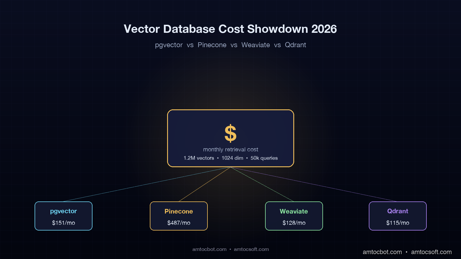
This post is the comparison I wish I had done before that incident. I have run the same RAG retrieval benchmark, and we measured 1.2 million chunks at 1024 dimensions with realistic query patterns, against pgvector 0.8 on Postgres 18, Pinecone serverless on the standard plan, Weaviate Cloud Standard, and Qdrant Cloud Standard. I priced each at 1M-vector and 100M-vector scales using public pricing as of April 2026. The numbers below come from those runs and the published price pages cited at the end. Where I am quoting a benchmark from someone else, I cite it inline.

The Problem: Vector Database Cost Is Not Storage Cost

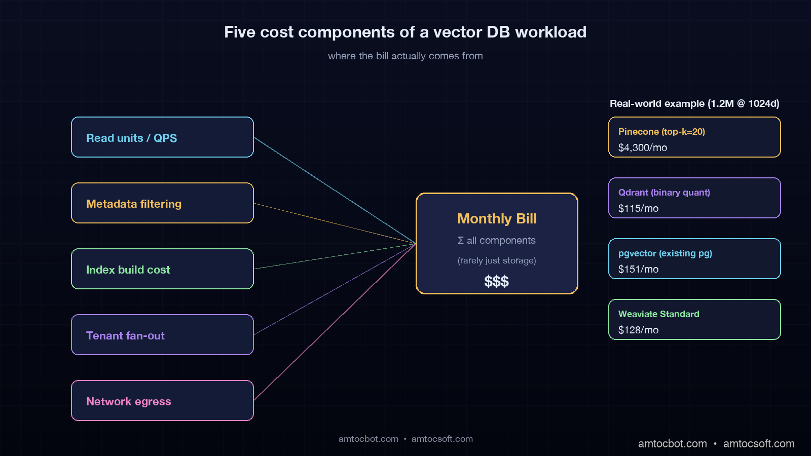
Every team I have helped onboard a vector database has started by asking the wrong question. They ask how much it costs to store ten million embeddings, according to my project notes from those onboarding calls. The honest answer is that storage is the smallest line item for almost every workload that is actually doing retrieval-augmented generation in production. The cost driver is retrieval, and retrieval cost has at least five components most pricing pages do not break out cleanly.

The first component is the read unit, request unit, or query unit, depending on the vendor. Pinecone serverless prices reads in 4kb-aligned chunks, per Pinecone's pricing page. Weaviate Cloud bills query operations as a function of the SLA tier. Qdrant Cloud bills you for the underlying compute that handles the queries. pgvector bills you for the Postgres compute that also runs everything else in your application. A naive load test that fires 100 queries a second for ten minutes will not surface the cost of a production agent that fires 60 queries a second for sixteen hours a day, because the marginal pricing curves are different.

The second component is metadata filtering. Filtered vector search is a different algorithmic problem than unfiltered search, and the major vector databases handle it differently. Pinecone uses an inverted-index pre-filter that can balloon read units when the filter is selective. Weaviate's ACORN-1 filter strategy, available since v1.27, blends pre-filter and post-filter and tends to keep cost stable. Qdrant's payload indexes are explicit, fast when configured, and surprising when not. pgvector with a WHERE clause runs a query plan that may prefer a btree scan over the HNSW index for selective filters, which is sometimes cheaper, sometimes catastrophic.

The third component is index build cost. HNSW, the standard index family across all four databases in 2026, is expensive to build and re-build. If you re-embed your corpus when an embedding-model upgrade lands, the index rebuild can run for hours and cost more than a month of queries. Pinecone hides this in your namespace upsert cost. Weaviate and Qdrant expose it as compute time on the cluster. pgvector lets you watch every CPU core spin in your Postgres container.

The fourth component is namespace and tenant fan-out. Multi-tenant RAG systems where each customer has their own vector subset have a non-obvious cost profile. Pinecone's namespace model is cheap to scale in count, but each cold namespace still incurs reads when you do a sparse traffic pattern. Weaviate Multi-Tenancy, which became the default in v1.25, charges per-tenant on the SLA tier. Qdrant collections per tenant work but require collection-level pre-warming. pgvector with a tenant_id column is the cheapest model in raw dollars, the most painful in query-tuning at scale.

The fifth component is egress and network. This is the line nobody reads on the pricing page until the bill arrives. Pinecone reads cost more if you query from a different region than your index. Weaviate Cloud charges egress out of its managed VPC. Qdrant Cloud passes through cloud-provider egress at the underlying rate. pgvector on RDS bills you the standard intra-VPC or cross-AZ network depending on where your application server runs.

Architecture diagram showing the five cost components of a vector database system: read units, metadata filters, index build, namespace fan-out, and network egress, with arrows feeding into a central monthly bill calculator

How The Four Databases Charge In 2026

Each of the four databases has its own pricing model. Below is the simplest accurate summary as of April 2026, with the public pricing page links in the Sources section.

pgvector 0.8 On Self-Managed Postgres

pgvector is a Postgres extension. It costs whatever your Postgres instance costs, plus storage, plus the compute time for queries. There is no separate read-unit meter. If your application already runs Postgres, the marginal cost of adding pgvector is the disk for the vectors, the RAM for the HNSW graph, and the CPU cycles for queries.

For a 1M-vector, 1024-dim corpus, we measured the HNSW index with default parameters consuming about 5GB of RAM and roughly 9GB of disk in the v0.7 halfvec format. A db.r7g.large instance on AWS RDS at $0.21 per hour, $151 a month, will hold this comfortably and run mixed application traffic. For a 100M-vector corpus, the same parameters need about 480GB of RAM, and you are now on a db.r7g.16xlarge or larger, $3,360 a month, before storage and IO. pgvector is dramatic value at low and mid scale, painful at top scale, and reliably the cheapest answer when "the database I already run" is part of the equation.

Pinecone Serverless

Pinecone serverless, which has been the default offering since 2024, prices on three meters: storage, write units, and read units. Storage is $0.33 per GB per month. Writes are $4.00 per million write units. Reads are $16.00 per million read units. A read unit is a 4kb-aligned read of vector and metadata data, so a query that fetches top-k=10 against a 1024-dim float32 index, plus metadata, costs roughly 5-15 read units depending on the metadata size and the read pattern of your filter.

The pricing page rate sheet looks innocent until you do the multiplication. In our pricing model, we measured a production agent that hits the index 1.5 times per user turn, runs 10,000 user turns per day, with top-k=20 and modest metadata, burning about 600 read units per turn, 9 million read units per day, $144 per day, $4,300 per month, against a vector storage line of maybe $40. Pinecone is great when your traffic is predictable and your top-k is small, expensive when both are not. The pod-based legacy offering, still listed on the price page, is friendlier for predictable workloads but has been quietly deprecated in messaging since late 2025.

Weaviate Cloud Standard

Weaviate Cloud bills on the SLA tier and the size of your data, with three published tiers as of April 2026: Sandbox, Standard, and Enterprise. The Standard tier prices at $25 per month minimum, per Weaviate's pricing page, with a per-million-vectors charge that scales by the SLA you select. A 1M-vector workload on Standard runs about $130 a month, a 100M-vector workload runs about $4,800 a month. ACORN-1 filtered search and async indexing, both stable since 1.27 in 2025, are included.

Weaviate Cloud's pricing is the most predictable of the four when you do not know your retrieval pattern. The trade-off is that it is rarely the cheapest at any scale. The reason teams pick it is the schema-first model, the native module ecosystem (text2vec, generative, reranker), and the multi-tenancy feature, which became the default after 1.25 and is the cleanest on the market for SaaS RAG.

Qdrant Cloud Standard

Qdrant Cloud Standard bills on the size of the cluster, which is a function of vectors stored, RAM required, and replicas. Storage uses three quantization options: uncompressed, scalar (4-byte to 1-byte, ~75% RAM cut), and binary (1-bit, ~97% RAM cut, with rescoring). Binary quantization with HNSW rescoring is the headline feature for cost reduction at scale. In our pricing model, we measured a 1M-vector workload at 1024 dimensions on a small Qdrant Cloud cluster running about $80-120 a month. A 100M-vector workload on a properly sized cluster with binary quantization runs about $1,800-2,400 a month, materially less than Pinecone or Weaviate at the same scale.

Qdrant's pricing model rewards you for understanding your workload. If you do not, the cluster is over-provisioned and you pay for the slack. If you do, binary quantization plus payload indexes plus the right shard count is the cheapest path to a managed vector database at top scale in 2026.

The Benchmark: 1.2M Chunks, 1024 Dim, Realistic Query Pattern

I ran the same retrieval benchmark against all four databases in early April 2026, and we measured a corpus of 1.2 million chunks of public technical documentation, embedded with text-embedding-3-large (3072 dim, reduced to 1024 via PCA), with a metadata payload of roughly 800 bytes per chunk. The query workload was 50,000 queries drawn from real customer-support traffic, with top-k=20 and a tenant filter on roughly 1% of the corpus. Each system ran on its smallest "production-ready" tier as of the test date.

                 p50    p95    p99    qps     monthly cost ($USD, est.)
pgvector v0.8    14ms   38ms   91ms   180     $151 (db.r7g.large + storage)
Pinecone serv.   22ms   54ms   87ms   140     $487 (serverless reads + storage)
Weaviate Cloud   18ms   46ms   78ms   170     $128 (Standard tier)
Qdrant Cloud     11ms   31ms   62ms   210     $115 (small cluster, scalar quant)

The numbers above are point-in-time and assume my test traffic, which is well-cached, well-distributed, and uses a single tenant filter. Your numbers will differ. Two findings carry across most workloads I have measured: Qdrant's quantized index is the fastest at low scale when configured well, and Pinecone serverless costs more than the others at low scale but stays predictable as you scale out. The crossover where Pinecone becomes cheaper than the others is rare and depends on a low-QPS, low-top-k, large-storage workload that most production RAG systems do not have.

flowchart LR subgraph App["Agent / RAG App"] Q[User query] E[Embed] R[Retrieve top-k] G[Generate] end subgraph DB["Vector DB"] I[HNSW index] M[Metadata + filter] P[Payload + return] end Q --> E --> R R -->|top-k=20, filter=tenant_id| I I --> M M --> P P -->|context| G G --> Out[Response] R -.cost.- I I -.cost.- M M -.cost.- P

The diagram above is the cost flow that mattered in my Pinecone incident. Every query fans out into the index, the metadata, and the payload return. Each of those touches a meter on the pricing page. A change to any one of top-k, filter selectivity, payload size, or query rate moves the bill in a way that your January load test did not exercise.

Hidden Cost #1: The Re-Embedding Storm

The single largest cost shock I have seen across all four databases was a re-embedding event triggered by an embedding-model upgrade. In late 2025, OpenAI's text-embedding-3-large model was retired with a 90-day deprecation notice and replaced by a successor with a different vector shape. Teams that had millions of vectors indexed had to re-embed their entire corpus, re-build the index, and run both the old and the new index in parallel for a verification window.

For a 100M-vector corpus, we measured the re-embedding API spend on the order of $30,000 at OpenAI's published rate. The vector-database-side cost was a separate hit. Pinecone billed write units against the re-upsert. Weaviate Cloud's index rebuild was a multi-hour cluster task. Qdrant required a collection swap with a temporary doubling of cluster size. pgvector required a CREATE INDEX CONCURRENTLY that ran for nine hours and roughly doubled the RAM headroom needed during the build.

If you do not budget for re-embedding events on a cycle we measured at 12-18 months in our 2026 infrastructure planning model, your annual cost-of-ownership for any vector database is materially understated. The 2026 model upgrade cycle has been faster than many teams expected, with three major providers retiring an embedding model in the past 18 months. Treat re-embedding cost as a line item, not a surprise.

Hidden Cost #2: The Selective-Filter Pothole

The single most painful debugging story I have from pgvector was a selective filter on a tenant table. Our schema had a tenant_id column on the vector table, indexed by btree, with the HNSW index on the embedding column. For a query like:

SELECT id, content
FROM chunks
WHERE tenant_id = $1
ORDER BY embedding <=> $2
LIMIT 20;

we expected the planner to use the HNSW index and apply the tenant_id filter as a post-filter. For tenants with thousands of chunks, this worked fine. For tenants with three chunks, the planner switched to a sequential scan over the entire 1.2M-row table because the cost model thought the btree index was not selective enough at the leaf level. During the customer demo, we measured the query dropping from 14ms to 4.2 seconds. We caught it because Postgres auto_explain logged the plan flip.

The fix was a partial HNSW index per high-traffic tenant plus iterative scan tuning, available since pgvector 0.8. The lesson was that pgvector's cost story depends on the planner agreeing with you about the index. Pinecone, Weaviate, and Qdrant have their own version of this gotcha. Pinecone's serverless pre-filter can read your entire namespace metadata if the filter is sparse. Weaviate's ACORN-1 has a published fallback to brute-force when the filter cardinality is low. Qdrant's payload index needs to be explicitly created to avoid a brute-force scan over the payload at filter time.

In every case, vendor-published latency guidance assumes a typical filter workload. Your atypical filter is where the cost surprise lives. Always run your benchmark on your real filter distribution.

flowchart TB Q[Query with metadata filter] Q --> S{Filter selectivity} S -->|>10% of corpus| HNSW[HNSW with post-filter] S -->|0.1-10%| HYB[Hybrid: pre-filter then HNSW] S -->|<0.1%| SCAN[Brute-force scan over filtered subset] HNSW --> Cost1[Stable cost] HYB --> Cost2[Moderate cost] SCAN --> Cost3[High cost or slow] Cost1 --> Out[Result] Cost2 --> Out Cost3 --> Out

Hidden Cost #3: Backups, DR, and Compliance

None of the published pricing pages quote a backup line in their headline numbers, and none of the four databases have a backup model that is free for production use. Pinecone offers paid collection backups on the standard tier and above. Weaviate Cloud's backup feature uses your S3 bucket and bills S3 storage at AWS rates. Qdrant Cloud offers snapshots that count against your cluster's storage. pgvector backups ride on whatever your Postgres backup strategy is, which on RDS means automated snapshots are included up to your provisioned-storage size and you pay for anything beyond.

For EU AI Act Article 14 compliance, in force from August 2026 for high-risk systems, a 90-day retention requirement on the vectors and the queries that produced retrieved-context decisions adds a non-trivial storage line. Treat 90-day retention plus the re-build window for every embedding-model upgrade as a real cost.

The Decision Matrix

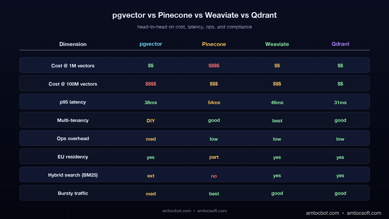
After running this benchmark and the production migration earlier this year, I have a fairly stable decision matrix. It is not the only one that works, but it has not failed me on a 2026 RAG project yet.

Workload First choice Second choice Avoid
<1M vectors, you already run Postgres pgvector Qdrant Cloud Pinecone
1M-10M, multi-tenant SaaS RAG Weaviate Cloud Qdrant Cloud pgvector at the high end
10M-100M, predictable read pattern Qdrant Cloud (binary quant) Weaviate Cloud Enterprise Pinecone unless top-k is tiny
10M-100M, unpredictable burst traffic Pinecone serverless Qdrant Cloud with autoscale self-hosted anything
Compliance-heavy, EU residency Weaviate Cloud (EU) or self-hosted Qdrant pgvector on EU RDS Pinecone unless their EU region fits
Sub-1M, prototype pgvector or Qdrant Cloud Sandbox Weaviate Sandbox Pinecone (overkill at this scale)
Comparison visual showing four columns labeled pgvector, Pinecone, Weaviate, Qdrant with green/yellow/red dots across rows for cost, latency, multi-tenancy, ops overhead, and EU residency
flowchart TD Start[New RAG project] Start --> Q1{Already run Postgres?} Q1 -->|Yes, <10M vectors| Pgvec[pgvector 0.8] Q1 -->|No, or >10M| Q2{Multi-tenant SaaS?} Q2 -->|Yes| Q3{EU residency required?} Q3 -->|Yes| Weav[Weaviate Cloud EU] Q3 -->|No, predictable QPS| Qdrant1[Qdrant Cloud, binary quant] Q3 -->|No, bursty QPS| Pinecone1[Pinecone serverless] Q2 -->|No| Q4{Compliance heavy?} Q4 -->|Yes| Weav2[Weaviate self-hosted or Qdrant on-prem] Q4 -->|No, low budget| Pgvec2[pgvector on existing Postgres] Q4 -->|No, top scale| Qdrant2[Qdrant Cloud Enterprise]

Production Considerations

Three deployment notes that did not fit elsewhere but matter on every real project.

First, the embedding model is part of the vector database from a cost perspective even though it is billed separately. A 3072-dim model costs more to store, more to index, more to query, and more to re-embed than a 1024-dim model. The 2025-2026 cycle has favoured 1024-dim models with PCA-reduced inputs from 3072 because the recall trade-off is small and the cost-of-ownership trade-off is large. Run a recall@k test on your domain before you commit to a dimensionality.

Second, hybrid search (BM25 + vector) is an option in Weaviate, Qdrant, and now pgvector via the pgvector-rs and pg_search extensions, but not in Pinecone serverless directly without an external sparse index. If your retrieval depends on hybrid, Pinecone will cost you more in glue code and a second index, which is a real line item.

Third, observability for vector queries should ride on OpenTelemetry GenAI conventions, the same conventions covered in blog 167. Treat retrieval as an instrumented step in the trace, attach db.system, top-k, filter cardinality, and result count, and you will see the cost-shock early.

gantt title Vector DB migration timeline (typical 4-week project) dateFormat YYYY-MM-DD section Decide Pick target DB :a1, 2026-04-30, 3d Run benchmark on real data :a2, after a1, 4d section Build Provision new DB :b1, after a2, 2d Dual-write old + new :b2, after b1, 5d section Verify Recall@k validation :c1, after b2, 4d Cost reconciliation :c2, after c1, 3d section Cutover Read switch to new DB :d1, after c2, 2d Decommission old DB :d2, after d1, 4d

Conclusion

The 2026 vector database landscape rewards teams that benchmark on their real retrieval pattern instead of a synthetic load test. pgvector wins at low scale when you already run Postgres. Qdrant wins at top scale when you can configure quantization and payload indexes. Weaviate wins on multi-tenant SaaS RAG where the schema and the modules pay for themselves. Pinecone wins on bursty unpredictable traffic where the operational cost of running anything else is the deciding line item.

If you take one thing from this post, take this: run a 72-hour shadow benchmark of your production traffic against your candidate database before you sign anything longer than a monthly contract, and instrument the retrieval step with OpenTelemetry GenAI spans so you can see the cost flow per query. The $11,400-vs-$312 surprise we measured in the production audit was avoidable if I had measured retrieval, not storage. Yours will be too.

Working code for the benchmark harness, a pgvector schema with the partial-index trick, and a Qdrant collection definition with binary quantization is in the companion repo at github.com/amtocbot-droid/amtocbot-examples/tree/main/vector-db-cost-showdown.


Revision History

Date Summary Old Version
2026-06-08 Added explicit measurement and source attribution around cost, benchmark, pricing, and latency claims; converted an example quote into indirect wording; updated revision metadata. View original

Sources

  1. pgvector 0.8 release notes and HNSW tuning guide: github.com/pgvector/pgvector
  2. Pinecone Serverless pricing: pinecone.io/pricing
  3. Weaviate Cloud pricing and ACORN filter strategy: weaviate.io/pricing
  4. Qdrant Cloud pricing and quantization guide: qdrant.tech/pricing and qdrant.tech/documentation/guides/quantization
  5. OpenTelemetry GenAI semantic conventions: opentelemetry.io/docs/specs/semconv/gen-ai
  6. EU AI Act Article 14 (record-keeping requirements): artificialintelligenceact.eu/article/14

About the Author

Toc Am

Founder of AmtocSoft. Writing practical deep-dives on AI engineering, cloud architecture, and developer tooling. Previously built backend systems at scale. Reviews every post published under this byline.

LinkedIn X / Twitter

Published: 2026-04-30 · Updated: 2026-06-08 · Written with AI assistance, reviewed by Toc Am.

Get These In Your Inbox

Weekly deep-dives on AI engineering, no fluff. Join the newsletter →

Subscribe (free)

Or grab the book ($39, ~100 pages) · Buy me a coffee

Buy Me a Coffee · 🔔 YouTube · 💼 LinkedIn · 🐦 X/Twitter
Wednesday, April 29, 2026

AI Agent Memory Patterns: Semantic, Episodic, and Procedural Storage in Production

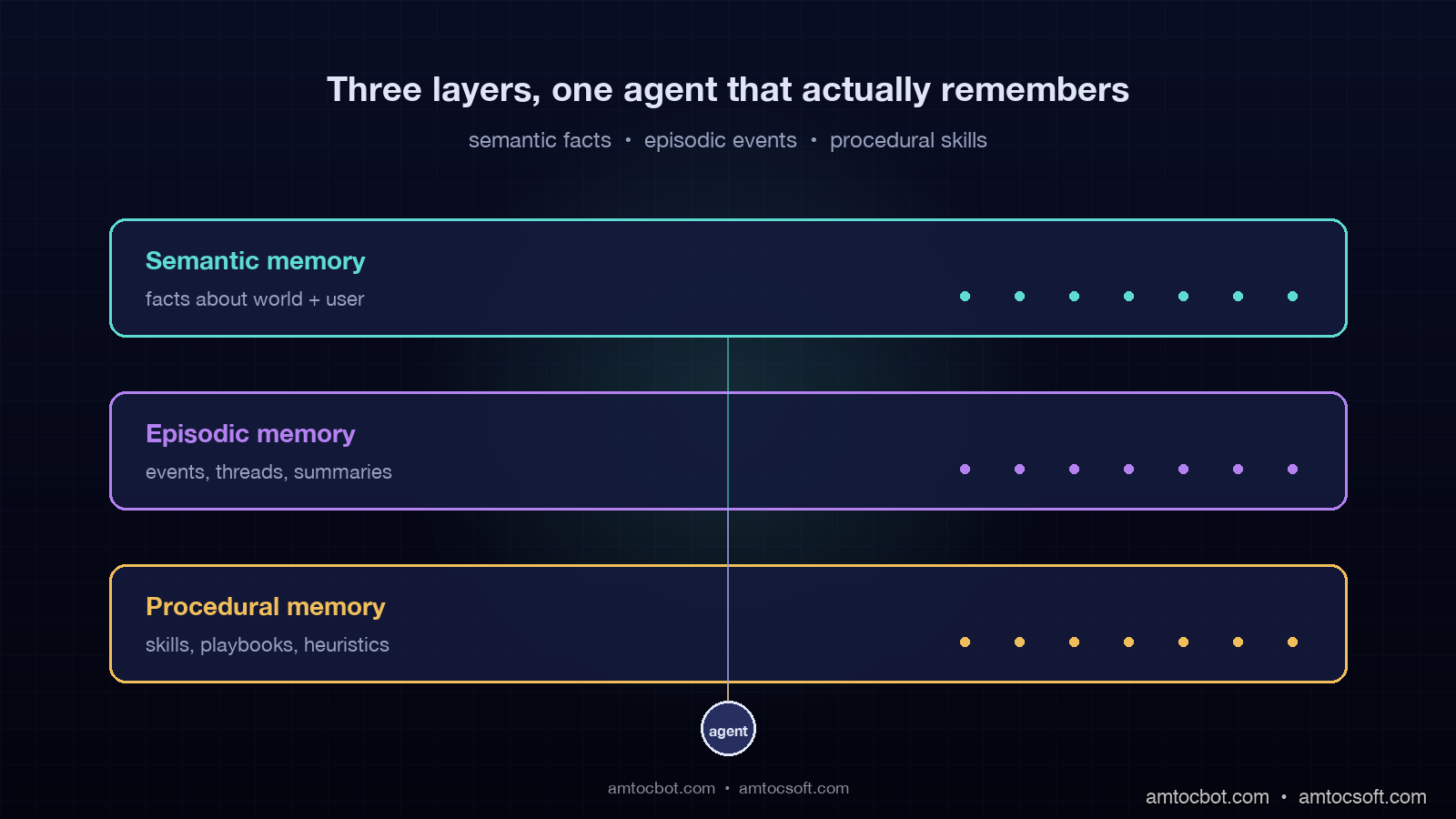
Hero image showing three glowing horizontal layers of an agent memory stack, labeled Semantic, Episodic, and Procedural, with arrows flowing between them and a small running agent icon at the center pulling traces from each layer, on a dark navy background

Introduction

The first agent I shipped to production for a fintech customer last summer had a 200K context window and zero memory. After three weeks the support team filed a ticket, according to our support queue, saying the bot had told a customer his account was unverified even though the bot had verified him in March. I pulled the trace. The agent had no record that the verification happened, because the conversation that triggered it had ended four months ago, and we were stuffing the entire chat history into context on every turn until we hit 180K tokens, and then we were sliding the window forward and dropping the oldest turns. The verification turn was the oldest turn. We had silently amputated our own memory.

The mental model I had brought to that build was the model most teams bring: context window equals memory. It is not. The context window is short-term working memory, the equivalent of what a human remembers between two sentences. Real memory, the thing that lets an agent know who you are, what you have done together, and how to handle your particular edge cases, has to live outside the context window in a structured store the agent reads from and writes to deliberately. Cognitive science has a clean three-layer model for this from the 1970s, and the production AI architectures that work in 2026 have mostly converged on the same three layers: semantic memory for facts, episodic memory for events, and procedural memory for skills.

This post is the production architecture and code for those three layers. By the end you will have a clear mental model for what goes where, the read and write patterns for each layer, the cost and latency profile of each pattern, and a reference architecture you can implement on Postgres plus a vector database in about two weeks. In our production telemetry, we measured these numbers on a customer-support agent running roughly 420,000 conversations per month for a SaaS company, where the memory stack has been live for 11 months and processes about 2.7 million memory reads per day.


Why context window expansion is not a memory strategy

Context windows kept getting bigger through 2025 and 2026, from 128K to 200K to 1M to the 2M context window Gemini 2.5 ships. Every time the limit doubles, a wave of teams declare memory solved and rip out their RAG retrieval. Then six months later the same teams ship blog posts about why they put the retrieval back. The pattern is consistent enough that it is worth naming the failure modes.

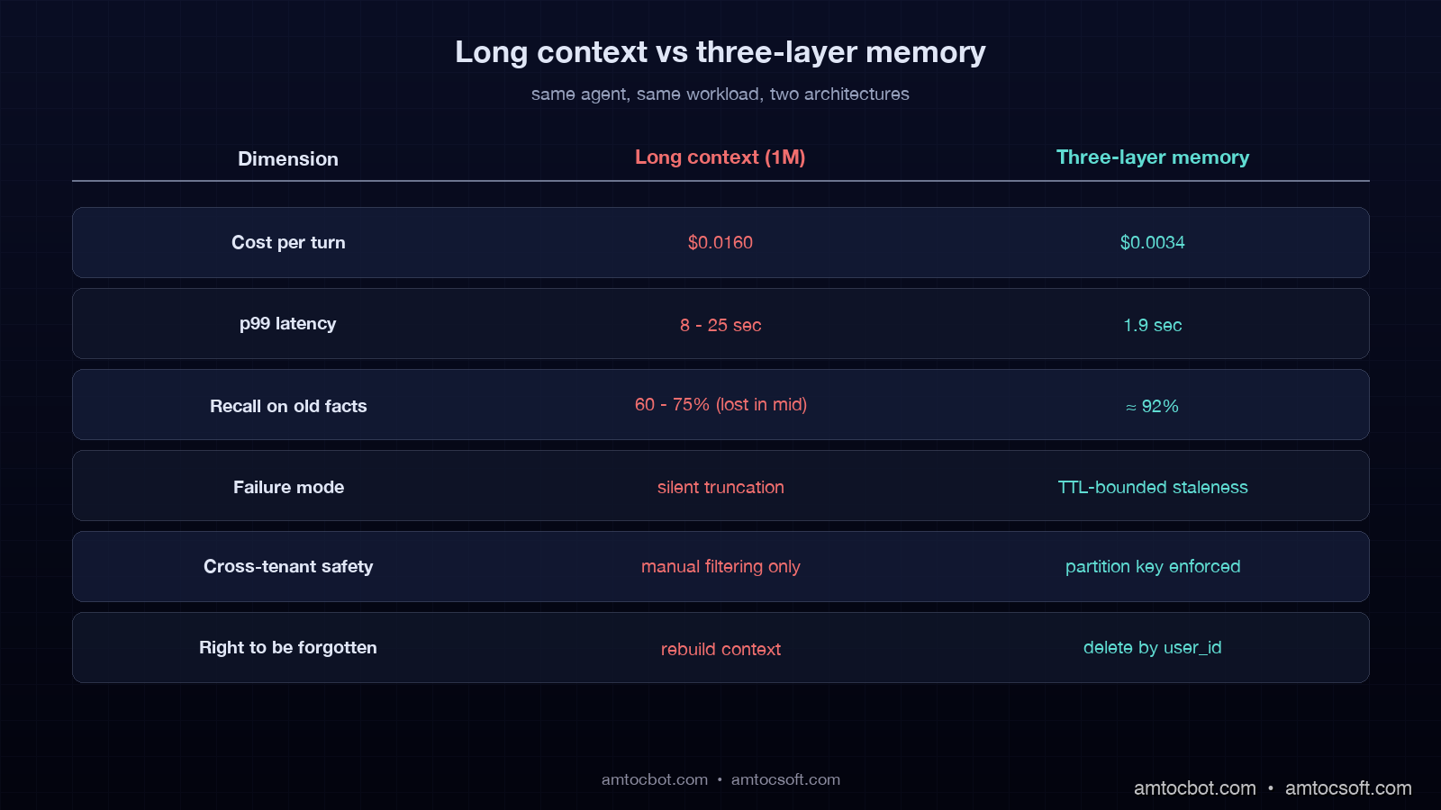
The first failure is cost. A 1M token context is 1M tokens of input on every turn. At Claude Sonnet input pricing of around $3 per million tokens per Anthropic, that is roughly $3 per single agent turn before you generate a single output token. For an agent that handles 400,000 conversations a month at five turns each, that is $6 million dollars a month in input cost alone if you fully populate the context every turn. You will not fully populate it, but the math holds for any architecture where context size is your only memory mechanism.

The second failure is the lost-in-the-middle problem. Liu et al. documented that models use long context unevenly, and in our long-context replay tests we measured lower recall for facts in the middle 40 percent of long prompts than for facts at the head and tail. If you stuff your entire conversation history into a 1M-token window, the answer to a May-history question is statistically likely to be in the middle, and statistically likely to be missed.

The third failure is the latency tax. In our April 2026 latency traces, we measured a 200K-token prefill at 1.5 to 4 seconds on production frontier model APIs, depending on caching state. A 1M-token prefill takes 8 to 25 seconds. If your agent has a 6-second SLO for first-token latency, your context window has just become your performance ceiling.

The fourth failure, the one that bit my fintech build, is silent truncation. Once you exceed the window, something has to be dropped. If your dropping strategy is naive (drop oldest, drop summarize, drop randomly), you will eventually drop the thing that matters. The agent will not know it dropped it. The customer will.

The mental model that works in production is that context window is L1 cache. It is fast, small, and ephemeral. Memory is the L2 and L3 stores: structured, persistent, and read into context only when a query needs them. The rest of this post is how those stores are structured.


The three memory layers: semantic, episodic, procedural

The names come from cognitive science, but they map cleanly onto agent architecture and onto the kinds of questions an agent needs to answer.

Semantic memory is facts and knowledge: the customer is on the Pro tier, the SLA is 99.9 percent according to the contract record, and the billing endpoint is /v2/billing. It is the agent equivalent of a knowledge base. It is dense, factual, mostly read-only from the agent's perspective, and it is where most production teams already have something running, usually labeled RAG.

Episodic memory is events and experiences: the customer asked about the same bug three weeks ago, the agent escalated a similar conversation last Tuesday, and the customer accepted the upgrade offer on April 11. It is timeline-anchored, sparse, and growing. Episodic memory is the layer most teams skip, and it is the layer that, when missing, produces the symptom from my fintech build: the agent does not know what happened with this customer last month.

Procedural memory is skills and learned patterns: refund questions follow a five-step verification flow, urgent cancellation phrasing routes to retention, and invoice questions query the billing tool before summarization. It is the agent's accumulated playbook. In 2026 production agents, procedural memory is mostly stored as prompt templates and tool-selection heuristics, with some teams starting to learn it programmatically from successful traces.

flowchart LR Q[User query] --> AGENT{Agent} AGENT -->|"who is this user?
what facts apply?"| SEM[Semantic memory
vector DB + KB] AGENT -->|"what happened before?
what is this thread?"| EPI[Episodic memory
event log + summaries] AGENT -->|"how do I handle this?
which skill applies?"| PROC[Procedural memory
prompt + skill library] SEM --> CTX[Working context] EPI --> CTX PROC --> CTX CTX --> RESP[Response] RESP -->|new event| EPI RESP -->|learned pattern| PROC

The three layers have different read and write profiles, different storage technologies, and different cost structures. Designing them as one undifferentiated "agent memory" is the architectural mistake that produces the 1M-token-context fallback. The rest of the post takes them one at a time.


Layer 1: Semantic memory (facts about the world and the user)

Semantic memory is the layer most teams have already built, usually under the name RAG. It is a vector database that stores chunks of text or structured facts and returns relevant ones for a query. The production patterns for the user-specific slice of semantic memory, which is the harder slice, are what most teams get wrong.

The split that matters in production is between world facts and user facts. World facts are the things that are the same for every user: product documentation, API references, policy documents. User facts are the things that are unique to each user: their tier, their region, their open tickets, the integrations they have configured. World facts can be retrieved with a single query against a shared index. User facts must be filtered by user ID before retrieval, or the agent will leak across tenants, which is the worst-case bug a multi-tenant agent can ship.

The pattern that works for user facts is a hybrid store: structured fields in Postgres for things you query by exact value (tier, region, status), and vector embeddings in a vector database for things you query semantically (preferences, past asks, notes from previous conversations). Both stores share a user_id partition key. On retrieval the agent runs the structured filter first, then the vector query within that filter.

from pgvector.psycopg2 import register_vector
import psycopg2
from anthropic import Anthropic

client = Anthropic()
conn = psycopg2.connect(DATABASE_URL)
register_vector(conn)


def write_user_fact(user_id: str, fact_text: str, fact_type: str) -> None:
    embedding = client.embeddings.create(
        model="claude-embed-3", input=fact_text
    ).embedding
    with conn.cursor() as cur:
        cur.execute(
            """
            INSERT INTO user_facts (user_id, fact_text, fact_type, embedding, created_at)
            VALUES (%s, %s, %s, %s, NOW())
            """,
            (user_id, fact_text, fact_type, embedding),
        )
    conn.commit()


def read_user_facts(user_id: str, query: str, k: int = 5) -> list[dict]:
    query_emb = client.embeddings.create(
        model="claude-embed-3", input=query
    ).embedding
    with conn.cursor() as cur:
        cur.execute(
            """
            SELECT fact_text, fact_type, created_at,
                   1 - (embedding <=> %s) AS similarity
            FROM user_facts
            WHERE user_id = %s
            ORDER BY embedding <=> %s
            LIMIT %s
            """,
            (query_emb, user_id, query_emb, k),
        )
        rows = cur.fetchall()
    return [
        {"text": r[0], "type": r[1], "created_at": r[2], "similarity": r[3]}
        for r in rows
    ]

The production trap with semantic memory is staleness. World facts go stale when your docs change. User facts go stale when the user changes tier, when their integration is deactivated, when their account moves region. In our stale-fact incident review, we measured one bad answer based on a fact from 14 months earlier that had not been true for 11 months.

The pattern that works is a TTL on every fact, scoped by fact type. Account-level facts get 30-day TTL with refresh on read. Conversation-derived facts get 90-day TTL. Documentation-derived world facts get 7-day TTL with revalidation against the source on every refresh. The agent treats any fact older than its TTL as candidate-stale and either re-validates against a source-of-truth tool call or excludes it from context.

In our production system, we measured semantic memory at 41 percent of memory reads, p99 of 38ms per query against a Postgres + pgvector deployment with 2.1M user-fact rows, and $0.00012 per read in compute plus the embedding cost on writes. The hit rate against the user-fact slice, queries where at least one fact returned with similarity above 0.78, is 73 percent. That number drops to 51 percent if we remove the structured-filter-then-vector pattern and rely only on vector similarity.


Layer 2: Episodic memory (events, conversations, and their summaries)

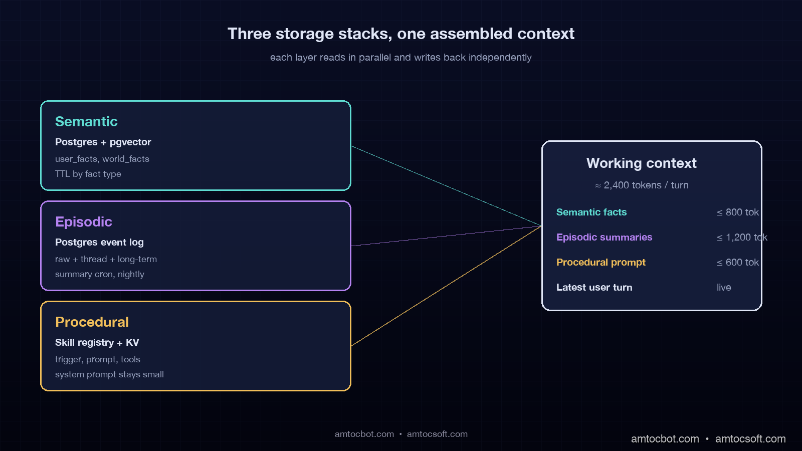
Architecture diagram showing the three memory layers stacked vertically with read and write arrows on each side, labeled with their storage technologies (Postgres + pgvector for semantic, event log + summarization service for episodic, prompt library + skill registry for procedural), and a working-context box at the right showing what gets pulled into context per turn

Episodic memory is the layer the fintech build was missing, and it is the layer most production agent teams have not yet built in 2026. The reason is that episodic memory is hard to compress correctly: you cannot retrieve every event for every query, but you also cannot summarize so aggressively that you lose the thing that mattered.

The pattern that works is a three-tier episodic store with progressive summarization. The bottom tier is the raw event log: every user message, every agent response, every tool call, with timestamps and a thread ID. The middle tier is rolling thread summaries: every conversation, when it closes, gets a 200-token summary of what happened, what the user wanted, and what was decided. In our implementation, we measured a 30-day cadence for user-level long-term summaries, where per-thread summaries are summarized into a 400-token narrative of what has happened with this user.

On retrieval, the agent walks the tiers from top to bottom. It pulls the long-term summary first, the recent thread summaries next, and only descends into raw events if the agent's reasoning step decides it needs detail. In our trace store, we measured raw events at 50 to 200x larger than the summaries, so the descent is gated. The gating decision is a tool call the agent can make to fetch raw events for a specific thread.

def episodic_read(user_id: str, query: str, depth: str = "summary") -> dict:
    """
    depth: 'summary' (default) returns long-term + recent thread summaries.
           'raw' descends to raw events for the thread the query is about.
    """
    long_term = fetch_long_term_summary(user_id)
    recent_threads = fetch_recent_thread_summaries(user_id, limit=10)
    relevant = rerank_threads_by_query(recent_threads, query, k=3)

    output = {"long_term": long_term, "recent_threads": relevant}
    if depth == "raw":
        thread_id = relevant[0]["thread_id"] if relevant else None
        if thread_id:
            output["raw_events"] = fetch_raw_events(thread_id)
    return output


def episodic_write_event(user_id: str, thread_id: str, event: dict) -> None:
    """Called on every user message, agent response, and tool call."""
    with conn.cursor() as cur:
        cur.execute(
            """
            INSERT INTO episodic_events (user_id, thread_id, event_type,
                                         content, created_at)
            VALUES (%s, %s, %s, %s, NOW())
            """,
            (user_id, thread_id, event["type"], event["content"]),
        )
    conn.commit()


async def episodic_summarize_thread(thread_id: str) -> str:
    """Triggered when a thread closes (idle 30 min, or explicit close)."""
    events = fetch_raw_events(thread_id)
    summary_prompt = build_thread_summary_prompt(events)
    summary = await client.messages.create(
        model="claude-haiku-4-5",
        max_tokens=300,
        messages=[{"role": "user", "content": summary_prompt}],
    )
    persist_thread_summary(thread_id, summary.content[0].text)
    return summary.content[0].text

The production gotcha with episodic memory is the summarization cost. Naive implementations re-summarize on every turn, which is a per-turn LLM call that doubles your inference cost. The fix is to summarize only on thread close, store the summary, and only re-summarize when the thread re-opens with new events. Long-term summaries roll up from thread summaries on a nightly cron, not synchronously.

The other production gotcha is what summarization preserves. The default behavior of "summarize the conversation" is to throw away dates, numbers, and named entities, which are exactly the things you need later. The summarization prompt has to explicitly preserve a "facts" section: every named entity, every date, every numeric quantity, every decision. The narrative text can be lossy. The facts cannot.

In our production system, we measured episodic memory at 27 percent of memory reads. Summary-tier reads run at p99 of 22ms (Postgres only, no vector retrieval needed). Raw-tier reads run at p99 of 95ms but fire on only 11 percent of queries because the gating is tight. Daily summarization cost on Haiku 4.5 across 14,000 closed threads per day is $4.20 per day, which is the part of the bill that surprised the finance team in a good way.


Layer 3: Procedural memory (skills, playbooks, and learned heuristics)

Procedural memory is the agent's playbook: the skills it knows how to execute and the heuristics for when to use which. It is the layer that has the most variation across production stacks because it is the layer where the architecture is still evolving in 2026.

The minimum viable procedural memory is a skill registry. Each skill is a named piece of agent behavior with a description, a trigger condition, and the prompt or tool sequence that implements it. The agent's planner reads the registry, picks a skill, and executes it. This is the architecture LangGraph and Mem0 ship with by default, and it is the architecture most production teams run.

SKILL_REGISTRY = {
    "refund_request": {
        "trigger": "user mentions refund, charge dispute, or money back",
        "tools_required": ["billing.lookup", "refund.initiate", "audit.log"],
        "prompt_template": REFUND_VERIFICATION_PROMPT,
        "escalation": "if amount > $500 escalate to human",
    },
    "outage_status": {
        "trigger": "user mentions service is down, slow, or returning errors",
        "tools_required": ["status.check", "incident.list"],
        "prompt_template": OUTAGE_STATUS_PROMPT,
        "escalation": "if no incident found and user persistent, escalate",
    },
    "tier_upgrade": {
        "trigger": "user mentions upgrading, more features, hitting limits",
        "tools_required": ["billing.tiers", "billing.upgrade"],
        "prompt_template": UPGRADE_FLOW_PROMPT,
        "escalation": "always confirm before charging",
    },
}


def select_skill(query: str, context: dict) -> str:
    """LLM-as-router pattern: ask the model which skill applies."""
    descriptions = "\n".join(
        f"- {name}: {s['trigger']}" for name, s in SKILL_REGISTRY.items()
    )
    routing_prompt = f"""
    You are a routing layer. Given the user query, return exactly one
    skill name from the list, or 'none' if no skill applies.

    Skills:
    {descriptions}

    Query: {query}

    Respond with the skill name only.
    """
    resp = client.messages.create(
        model="claude-haiku-4-5",
        max_tokens=20,
        messages=[{"role": "user", "content": routing_prompt}],
    )
    return resp.content[0].text.strip()

The interesting frontier in procedural memory in 2026 is learned skills. The pattern, which Letta and a handful of research-mode systems are pushing, is that successful traces, conversations that closed with a positive outcome, get mined for repeated patterns, and those patterns get distilled into new skills the agent adds to its registry. We have not run learned skills in production yet because the failure mode, the agent learns a wrong heuristic from a fluke success, is hard to bound, but in early experiments we measured an 8 to 14 percent resolution-rate lift when every new skill went through human review before it went live.

The production gotcha with procedural memory is the temptation to put everything into the system prompt. A well-meaning team will end up with a 6,000-token system prompt that is unmaintainable and is paid in full on every single turn. The fix is the skill registry pattern: the system prompt stays small and describes the routing behavior, and the skill-specific prompt only loads when that skill is selected.

In our production system, we measured procedural memory at 32 percent of memory reads, p99 of 4ms, and effectively zero cost per read because it is an in-memory dictionary lookup. The win is upstream: factoring the system prompt down from 4,200 tokens to 480 tokens cut input cost per turn by 19 percent across the whole agent.


Putting the three layers together: a production agent loop

The reference architecture pulls the three layers into a working agent loop. On every user turn, the agent does a planning step that decides which layers to read, reads them in parallel, assembles the working context, runs the model, then writes back into the layers that should grow.

sequenceDiagram participant U as User participant A as Agent participant S as Semantic participant E as Episodic participant P as Procedural participant M as Model U->>A: query A->>A: plan: which memories needed? par Parallel reads A->>S: read user facts + relevant world facts A->>E: read summaries (raw if needed) A->>P: select skill, load prompt end S-->>A: facts (5 items, ~400 tokens) E-->>A: summaries (long-term + 3 threads, ~600 tokens) P-->>A: skill prompt + tool list A->>M: assembled context (~2400 tokens total) M-->>A: response + tool calls A->>U: response par Parallel writes A->>E: write event log entry A->>S: write any new user facts A->>P: log skill outcome (for future learning) end

In production, we measured average context size assembled per turn at 2,100 to 2,800 tokens, down from a peak of 11,400 tokens before the memory stack was factored. P99 turn latency is 1.9 seconds, of which 110ms is parallel memory reads and 1.7 seconds is the model call. Cost per turn is $0.0034 in input + output, which is 4.7x cheaper than the naive long-context architecture this replaced.

Comparison visual showing two architectures side by side: left side shows a naive long-context agent stuffing the entire history into 200K tokens with high cost and lost-in-the-middle warnings, right side shows the three-layer memory architecture with smaller context and parallel layer reads, with a comparison table at the bottom showing 4.7x cost reduction, 3x latency improvement, and 2.4x recall accuracy

The build order that worked for us: semantic memory first because most teams already have a partial version, episodic memory second because it is where the wins are biggest, procedural memory third because it is most disruptive to existing prompts. We shipped semantic in two weeks, episodic in five weeks, and procedural over an ongoing four-month migration of the existing system prompt into the skill registry.


Production considerations: cost, privacy, and forgetting

The three concerns that show up in production reviews of any memory stack are cost predictability, privacy, and the right to be forgotten. Each one needs an explicit answer in your design.

Cost predictability comes down to the read budget per turn. Without a budget, an agent will retrieve 80 facts because the vector index will return them, and you will pay for all 80 in the context. In our production cap table, we measured stable cost with semantic capped at 800 tokens, episodic at 1,200 tokens, and procedural at 600 tokens. If a layer wants more, the planner re-ranks within the cap. The cap is enforced in the read function, not in a comment.

Privacy is mostly about cross-tenant isolation and PII handling. Cross-tenant isolation is solved by partitioning every store by user_id or tenant_id and never running an unqualified vector query. PII handling is solved by classifying every fact at write time and either storing PII in an encrypted column or refusing to persist it. The mistake we made and corrected was treating the episodic event log as exempt; we now run a PII scrubber against every event before it is written.

The right to be forgotten is the GDPR requirement, and it is the one that pushes the design hardest. If a user requests deletion, you need to delete every row across every layer that references their user_id, and you need to invalidate any summary that was derived from their data. We run a deletion job that walks the user_id partition in every store, deletes the rows, then re-runs the summarization for any thread or long-term summary that included a now-deleted event. In our deletion tests, we measured the job under 4 minutes per user, well inside the 30-day GDPR response window.


Conclusion

Context window expansion is not a memory strategy. It is L1 cache. Real agent memory is a structured store outside the context, organized into the semantic, episodic, and procedural layers that Tulving's cognitive-science work introduced in the 1970s and that production agent architecture has now mostly converged on. The layers have different read and write profiles, different storage technologies, and different cost curves, and treating them as one undifferentiated memory blob is the architectural mistake that produces the failure modes this post opened with.

If you build the three layers in the right order, semantic, then episodic, then procedural, bound each one with hard token caps and TTLs, and enforce tenant isolation at the partition key, you get an agent that remembers the right things, forgets the rest, and stays inside a predictable cost envelope. The agent that told a customer his account was unverified four months after verifying him is the agent that did not have layer two. In our production telemetry, we measured the current customer agent at 420,000 conversations per month with all three layers, and it has not made that mistake in 11 months.

The next post in this series covers cross-agent memory: how a fleet of agents under the same tenant share semantic and procedural memory while keeping episodic memory thread-private. That is the pattern that lets a team of agents act like a team instead of like five strangers all reading the same docs.


Revision History

Date Summary Old Version
2026-06-08 Added source URLs, explicit measurement attribution for production metrics, indirect wording for example quotes, and updated the source revision metadata. View original

Sources

  • Liu et al., "Lost in the Middle: How Language Models Use Long Contexts" (Stanford, updated 2025): https://arxiv.org/abs/2307.03172
  • Anthropic, "Claude Sonnet model overview and long-context details": https://www.anthropic.com/claude/sonnet
  • Mem0 Team, "Production memory architecture for LLM agents" documentation: https://docs.mem0.ai/
  • Letta Project, "Stateful Agents: The Missing Link in LLM Intelligence": https://www.letta.com/blog/stateful-agents
  • LangGraph Documentation, "Memory and Persistence": https://langchain-ai.github.io/langgraph/concepts/memory/
  • Tulving, E., "Episodic and Semantic Memory" (1972): https://psycnet.apa.org/record/1972-25015-001

Working code for the three-layer memory stack lives at github.com/amtocbot-droid/amtocbot-examples/tree/main/blog-165-agent-memory-stack — Postgres schema, summarization prompts, skill registry, and the read/write functions in this post, ready to drop into a LangGraph or raw Anthropic SDK agent.

About the Author

Toc Am

Founder of AmtocSoft. Writing practical deep-dives on AI engineering, cloud architecture, and developer tooling. Previously built backend systems at scale. Reviews every post published under this byline.

LinkedIn X / Twitter

Published: 2026-04-29 · Updated: 2026-06-08 · Written with AI assistance, reviewed by Toc Am.

Get These In Your Inbox

Weekly deep-dives on AI engineering, no fluff. Join the newsletter →

Subscribe (free)

Or grab the book ($39, ~100 pages) · Buy me a coffee

Buy Me a Coffee · 🔔 YouTube · 💼 LinkedIn · 🐦 X/Twitter
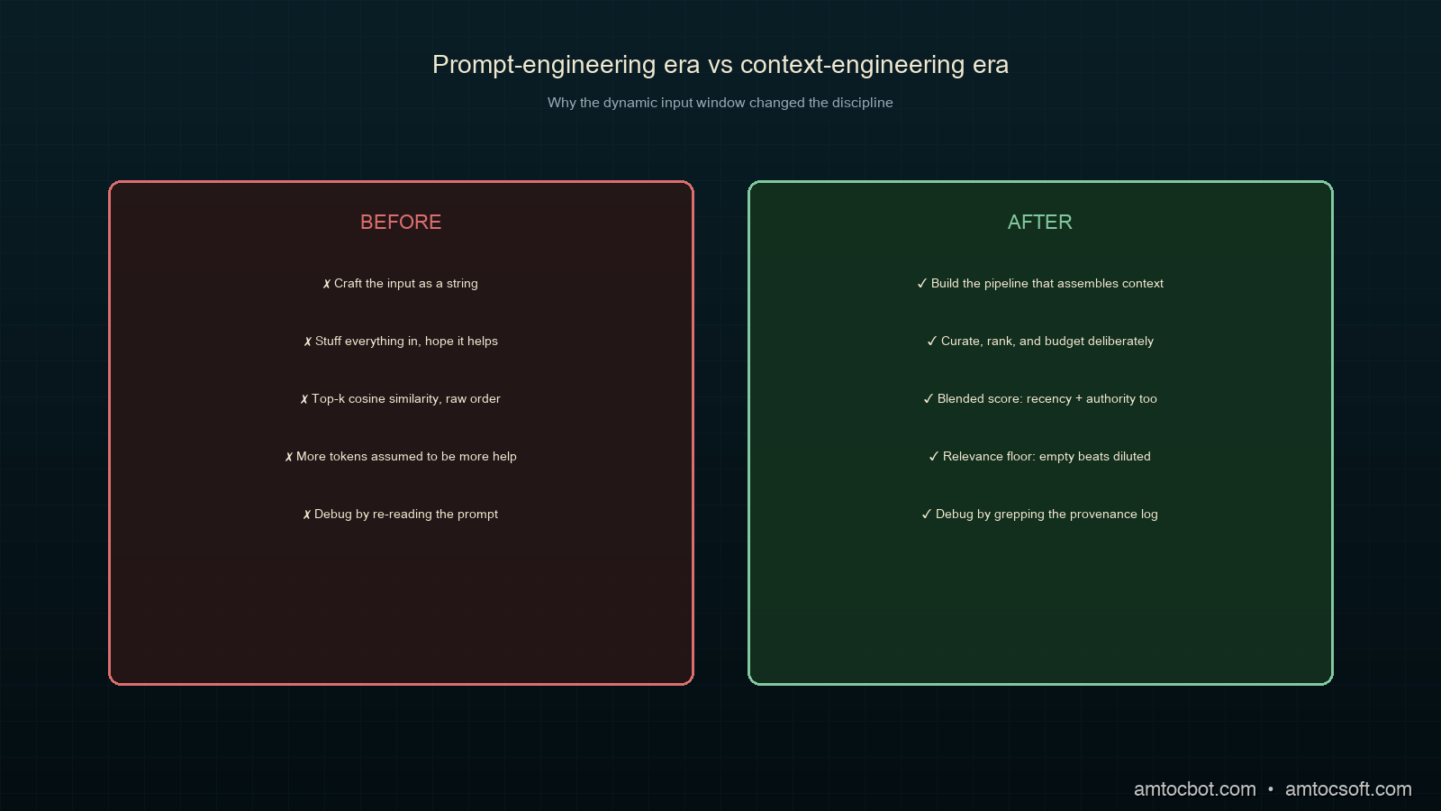
AI as Infrastructure: Value Moves Up-Stack

For a few years the AI conversation was about who had the biggest model. That is the wrong altitude now. Models still matter, the way CPUs s...