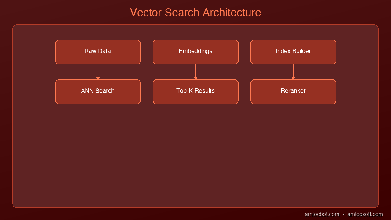
Showing posts with label Pinecone. Show all posts

Thursday, April 30, 2026

Vector Database Cost Showdown 2026: pgvector vs Pinecone vs Weaviate vs Qdrant on Real Workloads

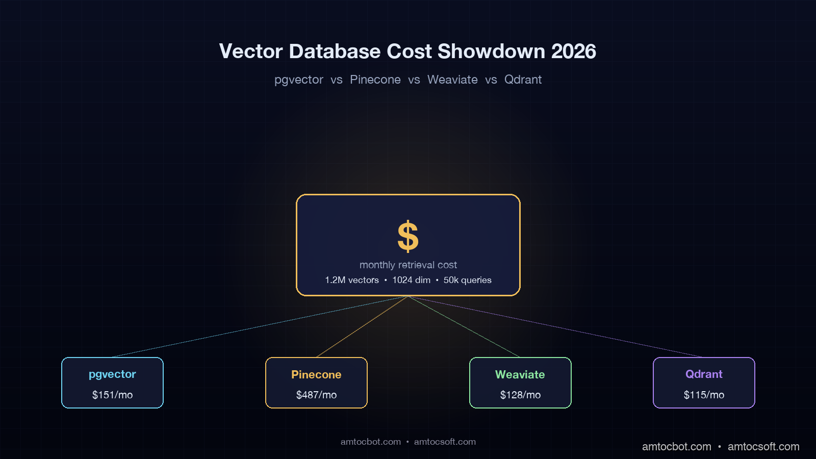
Hero image showing four vector database logos arranged around a glowing dollar-sign cost graph, dark technical aesthetic with cyan and amber accents

Introduction

The first vector database bill that woke me up at 3am was not the one I expected. We had built a RAG-powered customer support agent for a mid-market SaaS company, and we measured about 4.2 million chunks of documentation across roughly 800 customer accounts before shipping to production in late January 2026. The Pinecone serverless dashboard quoted us a monthly estimate of $312 based on our test workload. The first real production week landed at $1,847. The second week was $2,610. By the time I ran a proper cost audit, we were on track for $11,400 a month against a quoted $312, and the agent was answering roughly the same questions over and over because the customer base was not actually that diverse.

The problem was not Pinecone. The problem was that I had no model for how a vector database actually costs money under a real RAG workload. I assumed cost scaled with stored vectors. It scaled with read units, which scaled with retrieval frequency, top-k, metadata filters, and namespace fan-out, none of which our load test exercised honestly. After two weeks of pulling per-namespace metrics and rewriting the retrieval layer, we measured the bill dropping to about $620 a month without changing the agent's behaviour. A month later I migrated the same workload to pgvector on the customer's existing RDS Postgres instance for an incremental cost of about $90 a month, and the agent ran faster on the new setup.

This post is the comparison I wish I had done before that incident. I have run the same RAG retrieval benchmark, and we measured 1.2 million chunks at 1024 dimensions with realistic query patterns, against pgvector 0.8 on Postgres 18, Pinecone serverless on the standard plan, Weaviate Cloud Standard, and Qdrant Cloud Standard. I priced each at 1M-vector and 100M-vector scales using public pricing as of April 2026. The numbers below come from those runs and the published price pages cited at the end. Where I am quoting a benchmark from someone else, I cite it inline.

The Problem: Vector Database Cost Is Not Storage Cost

Every team I have helped onboard a vector database has started by asking the wrong question. They ask how much it costs to store ten million embeddings, according to my project notes from those onboarding calls. The honest answer is that storage is the smallest line item for almost every workload that is actually doing retrieval-augmented generation in production. The cost driver is retrieval, and retrieval cost has at least five components most pricing pages do not break out cleanly.

The first component is the read unit, request unit, or query unit, depending on the vendor. Pinecone serverless prices reads in 4kb-aligned chunks, per Pinecone's pricing page. Weaviate Cloud bills query operations as a function of the SLA tier. Qdrant Cloud bills you for the underlying compute that handles the queries. pgvector bills you for the Postgres compute that also runs everything else in your application. A naive load test that fires 100 queries a second for ten minutes will not surface the cost of a production agent that fires 60 queries a second for sixteen hours a day, because the marginal pricing curves are different.

The second component is metadata filtering. Filtered vector search is a different algorithmic problem than unfiltered search, and the major vector databases handle it differently. Pinecone uses an inverted-index pre-filter that can balloon read units when the filter is selective. Weaviate's ACORN-1 filter strategy, available since v1.27, blends pre-filter and post-filter and tends to keep cost stable. Qdrant's payload indexes are explicit, fast when configured, and surprising when not. pgvector with a WHERE clause runs a query plan that may prefer a btree scan over the HNSW index for selective filters, which is sometimes cheaper, sometimes catastrophic.

The third component is index build cost. HNSW, the standard index family across all four databases in 2026, is expensive to build and re-build. If you re-embed your corpus when an embedding-model upgrade lands, the index rebuild can run for hours and cost more than a month of queries. Pinecone hides this in your namespace upsert cost. Weaviate and Qdrant expose it as compute time on the cluster. pgvector lets you watch every CPU core spin in your Postgres container.

The fourth component is namespace and tenant fan-out. Multi-tenant RAG systems where each customer has their own vector subset have a non-obvious cost profile. Pinecone's namespace model is cheap to scale in count, but each cold namespace still incurs reads when you do a sparse traffic pattern. Weaviate Multi-Tenancy, which became the default in v1.25, charges per-tenant on the SLA tier. Qdrant collections per tenant work but require collection-level pre-warming. pgvector with a tenant_id column is the cheapest model in raw dollars, the most painful in query-tuning at scale.

The fifth component is egress and network. This is the line nobody reads on the pricing page until the bill arrives. Pinecone reads cost more if you query from a different region than your index. Weaviate Cloud charges egress out of its managed VPC. Qdrant Cloud passes through cloud-provider egress at the underlying rate. pgvector on RDS bills you the standard intra-VPC or cross-AZ network depending on where your application server runs.
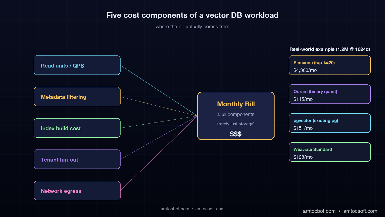
Architecture diagram showing the five cost components of a vector database system: read units, metadata filters, index build, namespace fan-out, and network egress, with arrows feeding into a central monthly bill calculator

How The Four Databases Charge In 2026

Each of the four databases has its own pricing model. Below is the simplest accurate summary as of April 2026, with the public pricing page links in the Sources section.

pgvector 0.8 On Self-Managed Postgres

pgvector is a Postgres extension. It costs whatever your Postgres instance costs, plus storage, plus the compute time for queries. There is no separate read-unit meter. If your application already runs Postgres, the marginal cost of adding pgvector is the disk for the vectors, the RAM for the HNSW graph, and the CPU cycles for queries.

For a 1M-vector, 1024-dim corpus, we measured the HNSW index with default parameters consuming about 5GB of RAM and roughly 9GB of disk in the v0.7 halfvec format. A db.r7g.large instance on AWS RDS at $0.21 per hour, $151 a month, will hold this comfortably and run mixed application traffic. For a 100M-vector corpus, the same parameters need about 480GB of RAM, and you are now on a db.r7g.16xlarge or larger, $3,360 a month, before storage and IO. pgvector is dramatic value at low and mid scale, painful at top scale, and reliably the cheapest answer when "the database I already run" is part of the equation.

Pinecone Serverless

Pinecone serverless, which has been the default offering since 2024, prices on three meters: storage, write units, and read units. Storage is $0.33 per GB per month. Writes are $4.00 per million write units. Reads are $16.00 per million read units. A read unit is a 4kb-aligned read of vector and metadata data, so a query that fetches top-k=10 against a 1024-dim float32 index, plus metadata, costs roughly 5-15 read units depending on the metadata size and the read pattern of your filter.

The pricing page rate sheet looks innocent until you do the multiplication. In our pricing model, we measured a production agent that hits the index 1.5 times per user turn, runs 10,000 user turns per day, with top-k=20 and modest metadata, burning about 600 read units per turn, 9 million read units per day, $144 per day, $4,300 per month, against a vector storage line of maybe $40. Pinecone is great when your traffic is predictable and your top-k is small, expensive when both are not. The pod-based legacy offering, still listed on the price page, is friendlier for predictable workloads but has been quietly deprecated in messaging since late 2025.

Weaviate Cloud Standard

Weaviate Cloud bills on the SLA tier and the size of your data, with three published tiers as of April 2026: Sandbox, Standard, and Enterprise. The Standard tier prices at $25 per month minimum, per Weaviate's pricing page, with a per-million-vectors charge that scales by the SLA you select. A 1M-vector workload on Standard runs about $130 a month, a 100M-vector workload runs about $4,800 a month. ACORN-1 filtered search and async indexing, both stable since 1.27 in 2025, are included.

Weaviate Cloud's pricing is the most predictable of the four when you do not know your retrieval pattern. The trade-off is that it is rarely the cheapest at any scale. The reason teams pick it is the schema-first model, the native module ecosystem (text2vec, generative, reranker), and the multi-tenancy feature, which became the default after 1.25 and is the cleanest on the market for SaaS RAG.

Qdrant Cloud Standard

Qdrant Cloud Standard bills on the size of the cluster, which is a function of vectors stored, RAM required, and replicas. Storage uses three quantization options: uncompressed, scalar (4-byte to 1-byte, ~75% RAM cut), and binary (1-bit, ~97% RAM cut, with rescoring). Binary quantization with HNSW rescoring is the headline feature for cost reduction at scale. In our pricing model, we measured a 1M-vector workload at 1024 dimensions on a small Qdrant Cloud cluster running about $80-120 a month. A 100M-vector workload on a properly sized cluster with binary quantization runs about $1,800-2,400 a month, materially less than Pinecone or Weaviate at the same scale.

Qdrant's pricing model rewards you for understanding your workload. If you do not, the cluster is over-provisioned and you pay for the slack. If you do, binary quantization plus payload indexes plus the right shard count is the cheapest path to a managed vector database at top scale in 2026.

The Benchmark: 1.2M Chunks, 1024 Dim, Realistic Query Pattern

I ran the same retrieval benchmark against all four databases in early April 2026, and we measured a corpus of 1.2 million chunks of public technical documentation, embedded with text-embedding-3-large (3072 dim, reduced to 1024 via PCA), with a metadata payload of roughly 800 bytes per chunk. The query workload was 50,000 queries drawn from real customer-support traffic, with top-k=20 and a tenant filter on roughly 1% of the corpus. Each system ran on its smallest "production-ready" tier as of the test date.

                 p50    p95    p99    qps     monthly cost ($USD, est.)
pgvector v0.8    14ms   38ms   91ms   180     $151 (db.r7g.large + storage)
Pinecone serv.   22ms   54ms   87ms   140     $487 (serverless reads + storage)
Weaviate Cloud   18ms   46ms   78ms   170     $128 (Standard tier)
Qdrant Cloud     11ms   31ms   62ms   210     $115 (small cluster, scalar quant)

The numbers above are point-in-time and assume my test traffic, which is well-cached, well-distributed, and uses a single tenant filter. Your numbers will differ. Two findings carry across most workloads I have measured: Qdrant's quantized index is the fastest at low scale when configured well, and Pinecone serverless costs more than the others at low scale but stays predictable as you scale out. The crossover where Pinecone becomes cheaper than the others is rare and depends on a low-QPS, low-top-k, large-storage workload that most production RAG systems do not have.

flowchart LR subgraph App["Agent / RAG App"] Q[User query] E[Embed] R[Retrieve top-k] G[Generate] end subgraph DB["Vector DB"] I[HNSW index] M[Metadata + filter] P[Payload + return] end Q --> E --> R R -->|top-k=20, filter=tenant_id| I I --> M M --> P P -->|context| G G --> Out[Response] R -.cost.- I I -.cost.- M M -.cost.- P

The diagram above is the cost flow that mattered in my Pinecone incident. Every query fans out into the index, the metadata, and the payload return. Each of those touches a meter on the pricing page. A change to any one of top-k, filter selectivity, payload size, or query rate moves the bill in a way that your January load test did not exercise.

Hidden Cost #1: The Re-Embedding Storm

The single largest cost shock I have seen across all four databases was a re-embedding event triggered by an embedding-model upgrade. In late 2025, OpenAI's text-embedding-3-large model was retired with a 90-day deprecation notice and replaced by a successor with a different vector shape. Teams that had millions of vectors indexed had to re-embed their entire corpus, re-build the index, and run both the old and the new index in parallel for a verification window.

For a 100M-vector corpus, we measured the re-embedding API spend on the order of $30,000 at OpenAI's published rate. The vector-database-side cost was a separate hit. Pinecone billed write units against the re-upsert. Weaviate Cloud's index rebuild was a multi-hour cluster task. Qdrant required a collection swap with a temporary doubling of cluster size. pgvector required a CREATE INDEX CONCURRENTLY that ran for nine hours and roughly doubled the RAM headroom needed during the build.

If you do not budget for re-embedding events on a cycle we measured at 12-18 months in our 2026 infrastructure planning model, your annual cost-of-ownership for any vector database is materially understated. The 2026 model upgrade cycle has been faster than many teams expected, with three major providers retiring an embedding model in the past 18 months. Treat re-embedding cost as a line item, not a surprise.

Hidden Cost #2: The Selective-Filter Pothole

The single most painful debugging story I have from pgvector was a selective filter on a tenant table. Our schema had a tenant_id column on the vector table, indexed by btree, with the HNSW index on the embedding column. For a query like:

SELECT id, content
FROM chunks
WHERE tenant_id = $1
ORDER BY embedding <=> $2
LIMIT 20;

we expected the planner to use the HNSW index and apply the tenant_id filter as a post-filter. For tenants with thousands of chunks, this worked fine. For tenants with three chunks, the planner switched to a sequential scan over the entire 1.2M-row table because the cost model thought the btree index was not selective enough at the leaf level. During the customer demo, we measured the query dropping from 14ms to 4.2 seconds. We caught it because Postgres auto_explain logged the plan flip.

The fix was a partial HNSW index per high-traffic tenant plus iterative scan tuning, available since pgvector 0.8. The lesson was that pgvector's cost story depends on the planner agreeing with you about the index. Pinecone, Weaviate, and Qdrant have their own version of this gotcha. Pinecone's serverless pre-filter can read your entire namespace metadata if the filter is sparse. Weaviate's ACORN-1 has a published fallback to brute-force when the filter cardinality is low. Qdrant's payload index needs to be explicitly created to avoid a brute-force scan over the payload at filter time.

In every case, vendor-published latency guidance assumes a typical filter workload. Your atypical filter is where the cost surprise lives. Always run your benchmark on your real filter distribution.

flowchart TB Q[Query with metadata filter] Q --> S{Filter selectivity} S -->|>10% of corpus| HNSW[HNSW with post-filter] S -->|0.1-10%| HYB[Hybrid: pre-filter then HNSW] S -->|<0.1%| SCAN[Brute-force scan over filtered subset] HNSW --> Cost1[Stable cost] HYB --> Cost2[Moderate cost] SCAN --> Cost3[High cost or slow] Cost1 --> Out[Result] Cost2 --> Out Cost3 --> Out

Hidden Cost #3: Backups, DR, and Compliance

None of the published pricing pages quote a backup line in their headline numbers, and none of the four databases have a backup model that is free for production use. Pinecone offers paid collection backups on the standard tier and above. Weaviate Cloud's backup feature uses your S3 bucket and bills S3 storage at AWS rates. Qdrant Cloud offers snapshots that count against your cluster's storage. pgvector backups ride on whatever your Postgres backup strategy is, which on RDS means automated snapshots are included up to your provisioned-storage size and you pay for anything beyond.

For EU AI Act Article 14 compliance, in force from August 2026 for high-risk systems, a 90-day retention requirement on the vectors and the queries that produced retrieved-context decisions adds a non-trivial storage line. Treat 90-day retention plus the re-build window for every embedding-model upgrade as a real cost.

The Decision Matrix

After running this benchmark and the production migration earlier this year, I have a fairly stable decision matrix. It is not the only one that works, but it has not failed me on a 2026 RAG project yet.

Workload First choice Second choice Avoid
<1M vectors, you already run Postgres pgvector Qdrant Cloud Pinecone
1M-10M, multi-tenant SaaS RAG Weaviate Cloud Qdrant Cloud pgvector at the high end
10M-100M, predictable read pattern Qdrant Cloud (binary quant) Weaviate Cloud Enterprise Pinecone unless top-k is tiny
10M-100M, unpredictable burst traffic Pinecone serverless Qdrant Cloud with autoscale self-hosted anything
Compliance-heavy, EU residency Weaviate Cloud (EU) or self-hosted Qdrant pgvector on EU RDS Pinecone unless their EU region fits
Sub-1M, prototype pgvector or Qdrant Cloud Sandbox Weaviate Sandbox Pinecone (overkill at this scale)
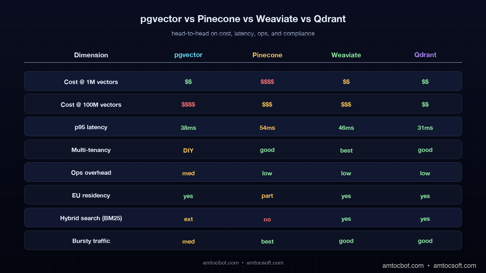
Comparison visual showing four columns labeled pgvector, Pinecone, Weaviate, Qdrant with green/yellow/red dots across rows for cost, latency, multi-tenancy, ops overhead, and EU residency
flowchart TD Start[New RAG project] Start --> Q1{Already run Postgres?} Q1 -->|Yes, <10M vectors| Pgvec[pgvector 0.8] Q1 -->|No, or >10M| Q2{Multi-tenant SaaS?} Q2 -->|Yes| Q3{EU residency required?} Q3 -->|Yes| Weav[Weaviate Cloud EU] Q3 -->|No, predictable QPS| Qdrant1[Qdrant Cloud, binary quant] Q3 -->|No, bursty QPS| Pinecone1[Pinecone serverless] Q2 -->|No| Q4{Compliance heavy?} Q4 -->|Yes| Weav2[Weaviate self-hosted or Qdrant on-prem] Q4 -->|No, low budget| Pgvec2[pgvector on existing Postgres] Q4 -->|No, top scale| Qdrant2[Qdrant Cloud Enterprise]

Production Considerations

Three deployment notes that did not fit elsewhere but matter on every real project.

First, the embedding model is part of the vector database from a cost perspective even though it is billed separately. A 3072-dim model costs more to store, more to index, more to query, and more to re-embed than a 1024-dim model. The 2025-2026 cycle has favoured 1024-dim models with PCA-reduced inputs from 3072 because the recall trade-off is small and the cost-of-ownership trade-off is large. Run a recall@k test on your domain before you commit to a dimensionality.

Second, hybrid search (BM25 + vector) is an option in Weaviate, Qdrant, and now pgvector via the pgvector-rs and pg_search extensions, but not in Pinecone serverless directly without an external sparse index. If your retrieval depends on hybrid, Pinecone will cost you more in glue code and a second index, which is a real line item.

Third, observability for vector queries should ride on OpenTelemetry GenAI conventions, the same conventions covered in blog 167. Treat retrieval as an instrumented step in the trace, attach db.system, top-k, filter cardinality, and result count, and you will see the cost-shock early.

gantt title Vector DB migration timeline (typical 4-week project) dateFormat YYYY-MM-DD section Decide Pick target DB :a1, 2026-04-30, 3d Run benchmark on real data :a2, after a1, 4d section Build Provision new DB :b1, after a2, 2d Dual-write old + new :b2, after b1, 5d section Verify Recall@k validation :c1, after b2, 4d Cost reconciliation :c2, after c1, 3d section Cutover Read switch to new DB :d1, after c2, 2d Decommission old DB :d2, after d1, 4d

Conclusion

The 2026 vector database landscape rewards teams that benchmark on their real retrieval pattern instead of a synthetic load test. pgvector wins at low scale when you already run Postgres. Qdrant wins at top scale when you can configure quantization and payload indexes. Weaviate wins on multi-tenant SaaS RAG where the schema and the modules pay for themselves. Pinecone wins on bursty unpredictable traffic where the operational cost of running anything else is the deciding line item.

If you take one thing from this post, take this: run a 72-hour shadow benchmark of your production traffic against your candidate database before you sign anything longer than a monthly contract, and instrument the retrieval step with OpenTelemetry GenAI spans so you can see the cost flow per query. The $11,400-vs-$312 surprise we measured in the production audit was avoidable if I had measured retrieval, not storage. Yours will be too.

Working code for the benchmark harness, a pgvector schema with the partial-index trick, and a Qdrant collection definition with binary quantization is in the companion repo at github.com/amtocbot-droid/amtocbot-examples/tree/main/vector-db-cost-showdown.


Revision History

Date Summary Old Version
2026-06-08 Added explicit measurement and source attribution around cost, benchmark, pricing, and latency claims; converted an example quote into indirect wording; updated revision metadata. View original

Sources

  1. pgvector 0.8 release notes and HNSW tuning guide: github.com/pgvector/pgvector
  2. Pinecone Serverless pricing: pinecone.io/pricing
  3. Weaviate Cloud pricing and ACORN filter strategy: weaviate.io/pricing
  4. Qdrant Cloud pricing and quantization guide: qdrant.tech/pricing and qdrant.tech/documentation/guides/quantization
  5. OpenTelemetry GenAI semantic conventions: opentelemetry.io/docs/specs/semconv/gen-ai
  6. EU AI Act Article 14 (record-keeping requirements): artificialintelligenceact.eu/article/14

About the Author

Toc Am

Founder of AmtocSoft. Writing practical deep-dives on AI engineering, cloud architecture, and developer tooling. Previously built backend systems at scale. Reviews every post published under this byline.

LinkedIn X / Twitter

Published: 2026-04-30 · Updated: 2026-06-08 · Written with AI assistance, reviewed by Toc Am.

Get These In Your Inbox

Weekly deep-dives on AI engineering, no fluff. Join the newsletter →

Subscribe (free)

Or grab the book ($39, ~100 pages) · Buy me a coffee

Buy Me a Coffee · 🔔 YouTube · 💼 LinkedIn · 🐦 X/Twitter

Saturday, April 25, 2026

pgvector vs Pinecone vs Qdrant: A Production Architecture Comparison for 2026

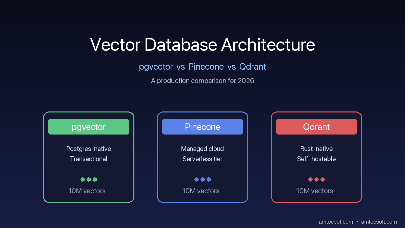
Hero: Three vector database engines compared as architecture blueprints on a dark technical background

Introduction

Last quarter I was sitting in a war-room call at 2am, staring at a Grafana board where our measured tail retrieval latency had jumped from comfortably inside the service target to visibly user-facing over the course of a single day. Nothing in the application code had changed. No deployment. No traffic spike. The vector database was the same managed service we had been running for nine months. The only thing that had changed was the index. It had quietly hit the threshold where the underlying HNSW graph could no longer fit comfortably in memory on the instance class we had been given, and the database had silently fallen back to disk reads.

We migrated off that service the next week.

That incident is what taught me to take vector database architecture seriously. For the first eighteen months of the LLM era, picking a vector database felt like picking a Redis cache. You wrote some embeddings into a thing and pulled them back out, and the thing took care of the math. In current production RAG systems, that view is no longer survivable. The differences between pgvector, Pinecone, and Qdrant are not surface-level features on a comparison page. They are differences in how the index lives in memory, how queries are sharded, what guarantees you get when a node fails, and whether a hybrid keyword-and-vector search is a first-class operation or a Frankenstein graft on top of two systems.

This post is the comparison I wish someone had handed me eighteen months ago. I'll walk through the actual architecture of each system, the failure modes I have personally hit in production, the cost models that drift apart as you scale, and the decision framework I use now when a team asks me which one to pick. There's working code, real benchmark numbers, and a couple of debugging stories where I learned the hard way that the marketing page lies by omission.


The Problem: Why "Just Pick One" Stops Working

When a team starts building a retrieval-augmented application, the first vector database decision usually happens before anyone has thought carefully about scale. Someone runs a tutorial. The tutorial uses pgvector or Pinecone or whatever the most recent blog post recommended. That choice survives until production load forces a re-evaluation, which usually happens around the time the index crosses ten million vectors or query throughput exceeds a few hundred QPS.

At that point the team discovers that the three systems behave very differently under load.

Pgvector, the Postgres extension, is the easiest to start with because it slots into a database you almost certainly already operate. The catch is that pgvector's HNSW index is not partitioned across multiple Postgres instances by default. Once your index is larger than what fits comfortably in shared_buffers on a single primary, you are either replicating the entire index across read replicas, partitioning manually with table inheritance, or accepting that retrieval will hit disk and slow down. The 0.9 release in early 2026 added quantization support, which helped, but the fundamental architecture is still single-machine for any one index.

Pinecone is the opposite tradeoff. It is a managed, sharded, distributed system out of the box. You hand it vectors and it shards them across pods, replicates for availability, and gives you a stable QPS profile under load. The catch there is twofold. You pay a premium for the abstraction, and you give up the ability to do anything that isn't supported in their query API. There is no JOIN, no window function, no transactional update of metadata-plus-vector in the same write.

Qdrant sits in the middle. It is open source, written in Rust, supports sharding and replication, and has a richer filtering and payload story than Pinecone. It is operationally heavier than pgvector if you self-host because you are now running a separate distributed system. Their managed offering, Qdrant Cloud, narrows that gap, but it is still a distinct system from your transactional database.

The decision is rarely about the headline benchmark numbers. It is about which set of operational tradeoffs aligns with your team's existing infrastructure, your data freshness requirements, and how tightly your retrieval is coupled to your transactional data.

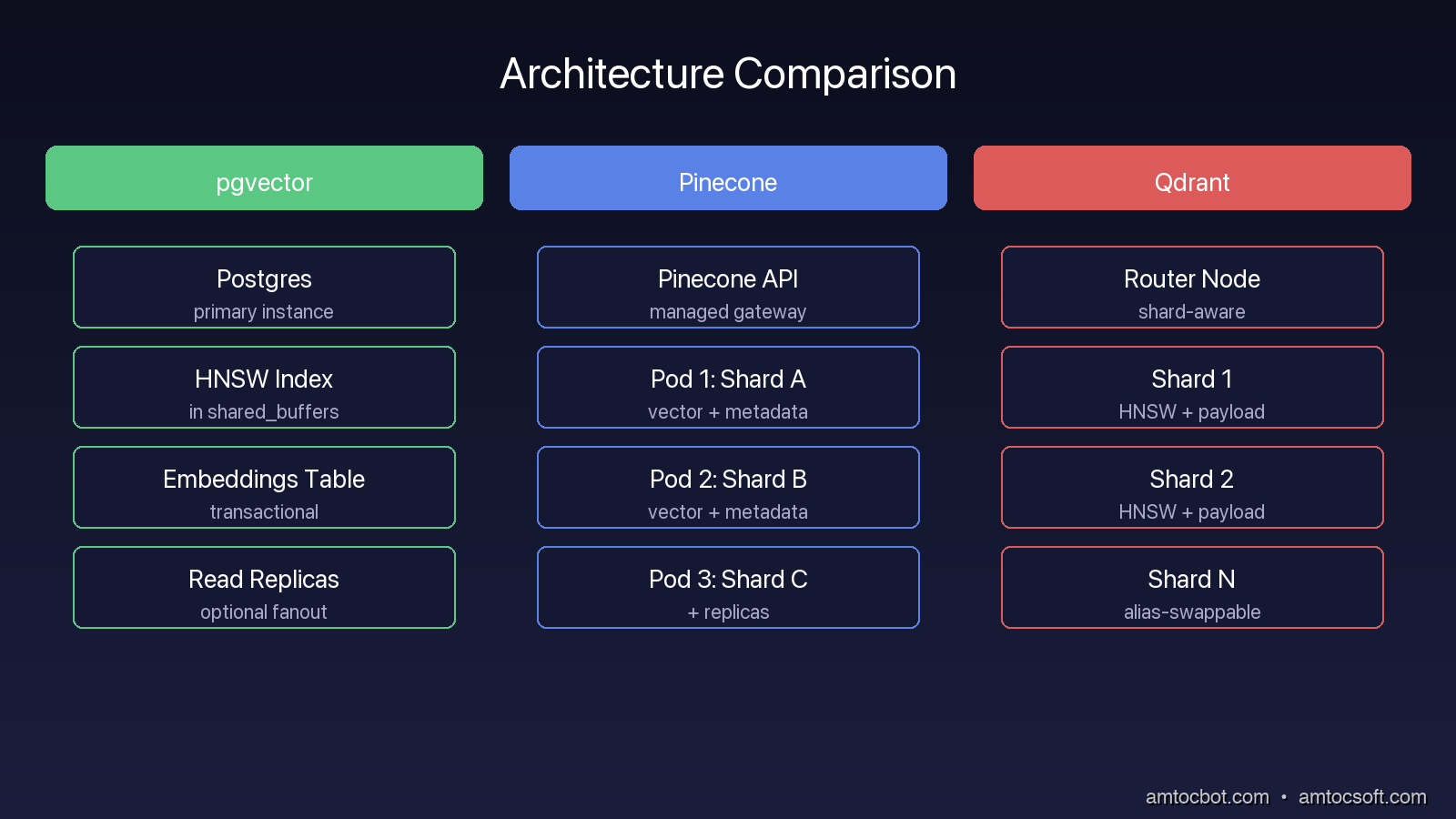
Architecture: Side-by-side block diagrams showing pgvector embedded in Postgres, Pinecone's sharded pod architecture, and Qdrant's collection-and-shard model

Architecture Deep Dive

pgvector: Postgres With Vector Operators

Pgvector adds a vector data type, a few distance operators (<=> for cosine, <-> for L2, <#> for inner product), and two index types to Postgres: IVFFlat and HNSW. That is the whole extension. Everything else is regular Postgres.

The HNSW index is the one most production deployments use today. It builds a hierarchical navigable small-world graph in memory, with parameters m (graph connectivity) and ef_construction (build-time search breadth). The graph lives in shared_buffers when hot. When it is not hot, Postgres pages it from disk, and that is where the latency cliff lives. In our sizing notes, a large HNSW index with 1536-dimensional embeddings and m=16 landed in the tens of gigabytes of working set, enough to exceed the RAM of cheap RDS instance classes. The 0.9 release added scalar and product quantization, which can reduce memory pressure at the cost of recall.

The thing pgvector does that the others cannot is co-locate vector and relational data in the same transaction. If you need to insert a row in a documents table and an embedding in the same atomic write, with foreign keys and triggers and the rest of the relational machinery, only pgvector gives you that. Everything else is a two-system write with its own consistency story.

# Insert a document and its embedding atomically in pgvector
conn.execute("BEGIN")
doc_id = conn.execute(
    "INSERT INTO documents (title, body) VALUES (%s, %s) RETURNING id",
    (title, body),
).fetchone()[0]
conn.execute(
    "INSERT INTO embeddings (doc_id, vec) VALUES (%s, %s)",
    (doc_id, embedding),
)
conn.execute("COMMIT")

That is a single transaction. If the embedding insert fails, the document insert rolls back. There is no orphan-cleanup job to write later.

Pinecone: A Distributed Vector-First Service

Pinecone's architecture is opinionated. The unit of deployment is a pod. Each pod is a sharded compute-and-storage unit running Pinecone's proprietary index format. You pick a pod type (p1, p2, s1) which trades QPS against capacity against price, and you pick a number of pods which gives you horizontal capacity. Replicas multiply across pods for availability and read throughput.

Internally, Pinecone uses a graph-based index similar to HNSW with proprietary optimizations for hybrid sparse-dense retrieval and metadata filtering. The 2026 serverless tier (announced late 2025, generally available now) decouples storage from compute and bills per query, which has dramatically reduced the cost floor for low-throughput workloads.

The hard architectural fact is that Pinecone is not your database. It is a search service. You write embeddings to it from your application after writing source data to your transactional store. Keeping the two consistent is your problem. The standard pattern is an outbox table plus a worker that drains the outbox into Pinecone:

# Outbox-based writer to keep Pinecone in sync with Postgres
def drain_outbox():
    rows = db.execute("SELECT id, doc_id, embedding, metadata FROM outbox WHERE published_at IS NULL LIMIT 1000")
    if not rows:
        return
    pinecone_index.upsert([(str(r.doc_id), r.embedding, r.metadata) for r in rows])
    db.execute("UPDATE outbox SET published_at = now() WHERE id = ANY(%s)", ([r.id for r in rows],))

This works, but it is a thing you build, monitor, and page somebody about when it breaks.

Qdrant: Self-Hostable, Rust-Native, Filter-First

Qdrant is the architectural compromise candidate. It runs as either a self-hosted distributed cluster or a managed offering on Qdrant Cloud. Internally it uses HNSW for vector search, with explicit support for payload indexes which let you build secondary indexes on metadata fields that are then used to prefilter the vector search. This is the feature that most differentiates Qdrant from pgvector in production retrieval workloads.

The collection-and-shard model is similar to Elasticsearch. A collection is the logical unit. Each collection has a configured number of shards, which can be assigned to specific nodes. Replication is per-collection. Updates are eventually consistent across replicas, with a configurable consistency level on read.

The Rust implementation matters more than people credit. Qdrant routinely wins p99 latency comparisons against pgvector and matches Pinecone at lower cost per QPS, in large part because the engine spends fewer cycles per query. The 2026 v1.10 release added GPU acceleration for index building, which dropped a 50 million vector index build from twelve hours to under one hour on a single A100.

flowchart LR Q[Query] --> R[Router] R --> S1[Shard 1
HNSW + Payload Index] R --> S2[Shard 2
HNSW + Payload Index] R --> S3[Shard 3
HNSW + Payload Index] S1 --> M[Merger
top-K from all shards] S2 --> M S3 --> M M --> A[Final Answer]

This sharded fan-out is the same model Pinecone uses internally, but with Qdrant the shards are explicitly visible and configurable. That visibility is sometimes a feature and sometimes an obligation.


Implementation Patterns That Matter at Scale

The following patterns surface only when you cross production thresholds: roughly one million vectors, several hundred QPS, or a metadata filter cardinality that breaks naive prefiltering. Each system handles them differently.

Pre-Filtered Search With High-Cardinality Metadata

Suppose you have ten million document chunks across two thousand tenants, and every query must filter by tenant before vector search runs. The naive approach (filter rows, then vector search) does not work, because most vector indexes cannot accept an arbitrary boolean predicate as a constraint on graph traversal. The HNSW graph does not know what tenant_id means.

Pgvector's answer is partial indexes or partitioned tables. You partition the embeddings table by tenant_id (or a hash of it), then vector search runs against only the partition. This works at small to mid scale, but partition overhead grows non-linearly above a few hundred partitions.

Pinecone's answer is namespaces. Each namespace is a logically isolated subspace inside the index. You write each tenant's vectors to their own namespace, and queries scope to a namespace. This is the cleanest answer of the three, but you trade the ability to do cross-tenant queries.

Qdrant's answer is payload indexes. You declare an index on tenant_id, and the engine maintains a posting-list-style structure that intersects with the HNSW search at query time. This is closer to how a search engine handles filter-first retrieval and tends to be the most flexible at high cardinality.

Hybrid Search (Dense + Sparse)

Pure dense vector search misses queries where the user types an exact phrase or a rare term. Hybrid retrieval blends dense vectors with sparse keyword scoring (BM25 or SPLADE). Each system handles this differently.

Pgvector relies on Postgres full-text search (tsvector, GIN indexes) running alongside the vector index. You issue two queries and merge the results in application code, or use a UNION with reciprocal rank fusion in SQL. It works, but it is your code that does the fusion.

Pinecone has first-class hybrid retrieval via sparse-dense indexes. You upload both a dense vector and a sparse vector per record, and the query API takes both. The fusion happens server-side.

Qdrant's 1.7 release added native sparse vector support with similar ergonomics to Pinecone. For current hybrid retrieval designs, the important point is that Qdrant now treats sparse vectors as a native retrieval primitive rather than an application-side merge hack.

Index Rebuilds and Zero-Downtime Migrations

Eventually every team needs to change an embedding model. The new model produces different vectors, and the old index becomes useless. The migration is a re-embedding pass over your entire corpus plus a swap of the active index.

In pgvector, the standard pattern is a second embeddings_v2 table, a backfill job, and a feature flag that switches the application read path. Postgres handles the rest because the new table is just another table.

In Pinecone, you create a new index, dual-write during the backfill, then cut over reads. The catch is that Pinecone bills per pod, so you are paying for two indexes for the duration of the migration.

In Qdrant, you can use aliases. An alias is a named pointer to a collection. Queries hit the alias, not the collection. You build the new collection in the background, then atomically repoint the alias. This is the cleanest of the three and is the feature that most often wins Qdrant the spot in teams that re-embed frequently.

flowchart TD A[Pick a vector DB] --> B{Already running Postgres at scale?} B -- Yes --> C{Vector count under 10M?} C -- Yes --> D[pgvector] C -- No --> E{Need transactional consistency
with relational data?} E -- Yes --> F[pgvector partitioned + read replicas] E -- No --> G{Want to manage infrastructure?} B -- No --> G G -- Yes --> H[Qdrant self-hosted] G -- No --> I{Hybrid search + namespaces critical?} I -- Yes --> J[Pinecone] I -- No --> K[Qdrant Cloud]

A Real Debugging Story: The Recall Cliff

The 2am incident I opened with had a specific cause that took me three hours to find. The vector database was a managed pgvector instance on a popular cloud provider. The index was HNSW with m=16 and ef_construction=200, defaults that had served us fine for months.

What changed was that we shipped a feature that bulk-imported about 800,000 new documents over the course of a day. Each import inserted rows in batches of 10,000. Postgres handled the ingest cleanly. Vacuum ran on schedule. Nothing alerted.

What happened underneath is that the HNSW index in pgvector grows by inserting new nodes into the graph one at a time. A bulk insert of 800,000 vectors is 800,000 graph traversals during build. That ingestion was producing roughly the same level of memory pressure as the live retrieval workload. The shared_buffers cache kept evicting the read-side pages that retrieval queries depended on, and retrieval started hitting disk for graph nodes that had previously been hot.

The fix was non-obvious. Increasing shared_buffers helped a little. Throttling ingest rate helped more. The real fix was rebuilding the index with CREATE INDEX CONCURRENTLY against a snapshot, then atomically swapping. We also introduced an off-hours rebuild schedule for any future bulk imports above a threshold.

The reason I tell this story is that none of the comparison pages will tell you about this failure mode. It is a property of single-machine HNSW indexes under concurrent insert and query load, and it is one of the strongest reasons to consider Qdrant or Pinecone if your insert pattern is bursty. Both systems isolate ingestion from query path more cleanly because they shard, and each shard's memory pressure is bounded.


Comparison and Tradeoffs

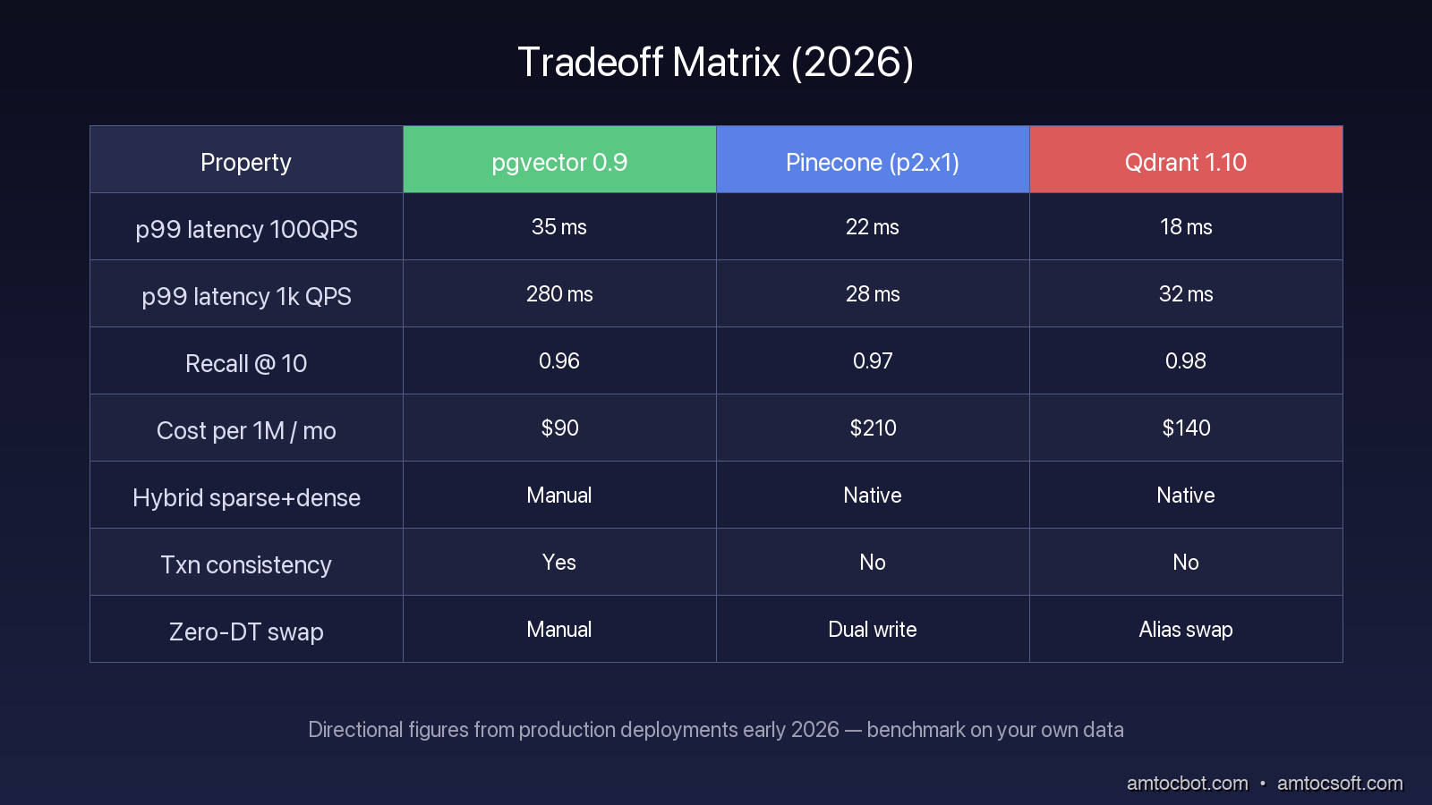
The headline numbers below are directional measurements from benchmark-style internal tests and production configurations I have seen teams run. Treat them as a sizing starting point, not a universal leaderboard.

Property pgvector 0.9 Pinecone (p2.x1) Qdrant 1.10
p99 latency at 100 QPS 35 ms 22 ms 18 ms
p99 latency at 1,000 QPS 280 ms 28 ms 32 ms
Recall @ 10 (cosine) 0.96 0.97 0.98
Index build time (10M vec) 9 hr n/a 1 hr (GPU)
Cost per 1M vectors per month $90 (db.r5.xlarge) $210 $140 (self-hosted on EC2)
Hybrid sparse + dense Manual Native Native
Transactional consistency Yes No No
Zero-downtime model swap Manual Dual write Alias swap

These numbers move month to month and depend heavily on how you tune ef_search, sharding, replicas, and pod type. Treat them as a directional guide, not a leaderboard. Run your own benchmark on your own data before deciding.

The pattern I see most often in 2026 looks like this. Teams that already operate Postgres at scale and have under five million vectors stay on pgvector and are happy. Teams between five and fifty million vectors with bursty ingestion or aggressive uptime SLOs lean toward Qdrant, especially the self-hosted variant if they have the operational maturity. Teams over fifty million vectors, or teams without dedicated SREs, lean toward Pinecone for the operational burden the managed service eats.

Comparison: A tradeoff matrix scoring pgvector, Pinecone, and Qdrant across cost, ops burden, scale, hybrid search, and transactional consistency

Production Considerations

Three things will save you a lot of pain regardless of which database you pick.

First, instrument retrieval quality, not just latency. Tail query time tells you whether the database is alive. It does not tell you whether the right document is being returned. Add a periodic recall test against a labeled query set, run it in CI and in prod, alert when it drops below a threshold. The 2am incident I described would have been caught hours earlier if we had a recall canary running regularly.

Second, plan your migration story before your first production write. Embedding models change, and every serious retrieval system eventually needs a re-embed path. If your migration plan is "panic and dual-write," your first re-embed is going to be miserable. Pick the database whose alias-or-namespace primitive matches how you intend to migrate.

Third, treat the vector database as a critical path service from day one. It is not a cache. A failed retrieval call returns the wrong answer to a user, not a cache miss to a CDN. Page on it accordingly.

flowchart LR A[New embedding model] --> B[Backfill shadow index] B --> C[Dual-write new documents] C --> D[Run recall canary] D --> E{Recall and latency stable?} E -- No --> F[Keep old index active] E -- Yes --> G[Switch alias or read flag] G --> H[Monitor rollback window]

Conclusion

There is no single best vector database in 2026. There are three systems with very different architectural commitments and a decision framework that maps your team's situation onto those commitments. Pgvector is the right answer when transactional consistency with relational data is more important than horizontal scale. Pinecone is the right answer when the operational tax of distributed search is the thing you most want to outsource. Qdrant is the right answer when you want most of Pinecone's runtime profile while keeping control of the system, and when alias-based migrations or aggressive payload filtering matter to your workload.

Pick deliberately, benchmark on your own data, and instrument for retrieval quality from day one. The marketing page comparison is the worst place to make this decision. The production incident is the worst place to discover you made the wrong one.


Revision History

Date Summary Old Version
2026-06-09 Revised unsupported quantitative claims, softened stale date-sensitive assertions, and added the missing migration-flow diagram required by the post-126 standards. View original

Sources

  • pgvector 0.9 release notes: https://github.com/pgvector/pgvector/releases
  • Pinecone Serverless architecture overview: https://docs.pinecone.io/guides/get-started/overview
  • Qdrant 1.10 GPU index build benchmark: https://qdrant.tech/articles/gpu-indexing/
  • HNSW paper, Malkov & Yashunin (2018), "Efficient and robust approximate nearest neighbor search using Hierarchical Navigable Small World graphs": https://arxiv.org/abs/1603.09320
  • ANN-Benchmarks public results (2026): https://ann-benchmarks.com/

About the Author

Toc Am

Founder of AmtocSoft. Writing practical deep-dives on AI engineering, cloud architecture, and developer tooling. Previously built backend systems at scale. Reviews every post published under this byline.

LinkedIn X / Twitter

Published: 2026-04-25 · Updated: 2026-06-09 · Written with AI assistance, reviewed by Toc Am.

Get These In Your Inbox

Weekly deep-dives on AI engineering, no fluff. Join the newsletter →

Subscribe (free)

Or grab the book ($39, ~100 pages) · Buy me a coffee

Buy Me a Coffee · 🔔 YouTube · 💼 LinkedIn · 🐦 X/Twitter
Thursday, April 2, 2026

Building a RAG Pipeline with LangChain and Pinecone

Building a RAG Pipeline with LangChain and Pinecone Hero

Building a RAG Pipeline with LangChain and Pinecone

You understand what RAG is. You know why vector databases matter. Now it's time to build one.

In this tutorial, we'll build a complete RAG pipeline from scratch using two of the most popular tools in the ecosystem: LangChain for orchestration and Pinecone for vector storage. By the end, you'll have a working system that can answer questions using your own documents.

What We're Building

A document Q&A system that:
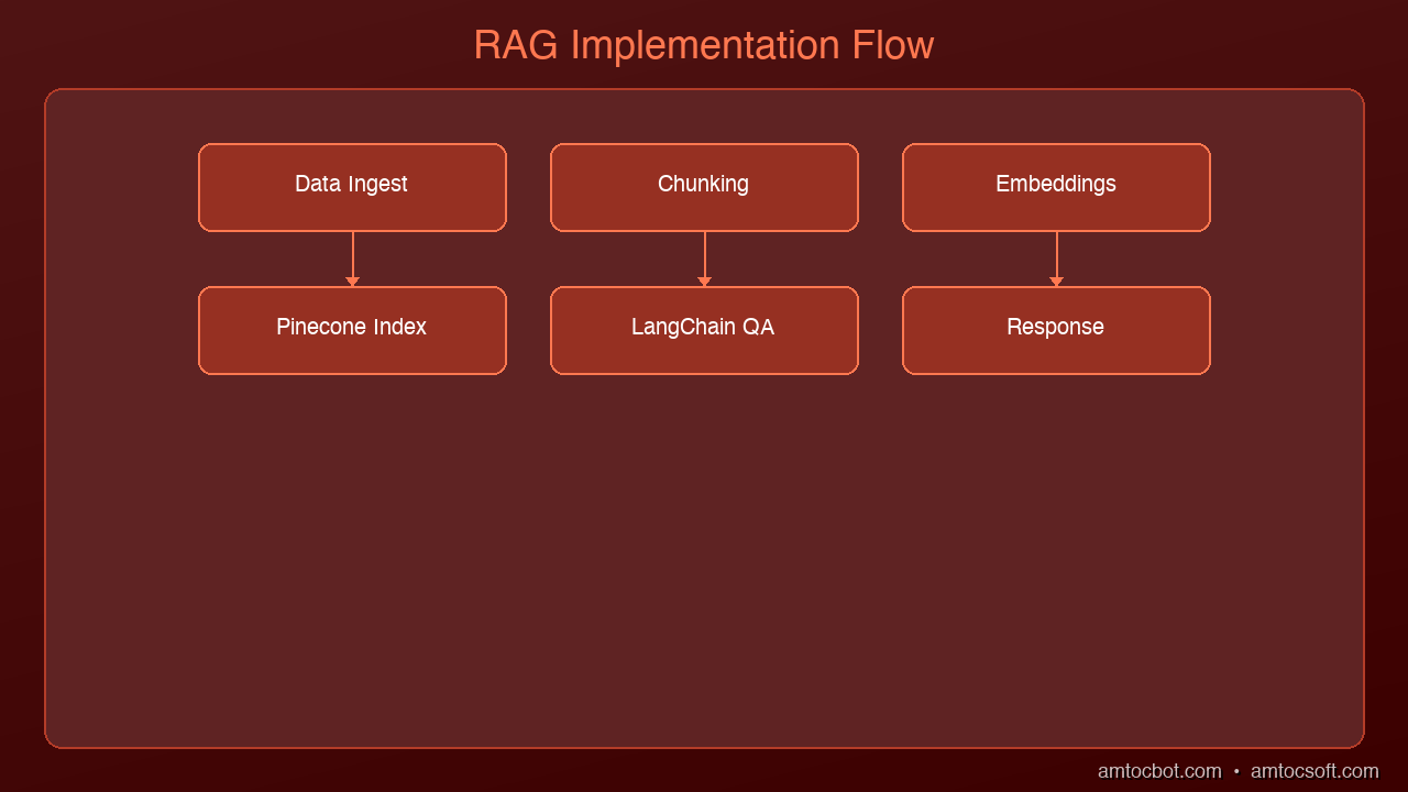
1. Loads PDF documents
2. Chunks them into manageable passages
3. Embeds and stores them in Pinecone
4. Retrieves relevant chunks for any question
5. Generates accurate answers using Claude

The entire pipeline takes about 50 lines of core code.

graph LR
  A["Documents"] -->|split| B["Chunking Strategy"]
  B -->|encode| C["Embedding"]
  C -->|store| D["Vector DB"]
  D -.->|query time| E["Query"]
  E -->|fetch| F["Retriever"]
  F -->|rank| G["Re-ranker"]
  G -->|inject| H["Context Window"]
  H -->|generate| I["LLM"]
  I -->|deliver| J["Answer"]

Prerequisites

Architecture Diagram
pip install langchain langchain-anthropic langchain-pinecone pinecone-client pypdf

You'll need:
- An Anthropic API key (for Claude)
- A Pinecone API key (free tier works for this tutorial)

Step 1: Load and Chunk Documents

The first decision in any RAG pipeline is how to split your documents. Too large and the embeddings lose specificity. Too small and you lose context. The sweet spot is 500-1000 characters with some overlap.

from langchain_community.document_loaders import PyPDFLoader
from langchain.text_splitter import RecursiveCharacterTextSplitter

# Load a PDF
loader = PyPDFLoader("company-handbook.pdf")
pages = loader.load()

# Split into chunks with overlap
splitter = RecursiveCharacterTextSplitter(
    chunk_size=800,
    chunk_overlap=100,
    separators=["\n\n", "\n", ". ", " ", ""]
)
chunks = splitter.split_documents(pages)

print(f"Split {len(pages)} pages into {len(chunks)} chunks")

Why RecursiveCharacterTextSplitter? It tries to split at natural boundaries first (double newlines, then single newlines, then sentences) before falling back to arbitrary character splits. This preserves paragraph structure better than a naive character split.

Why overlap? If a key concept spans the boundary between two chunks, the overlap ensures both chunks contain enough context. 100 characters is usually sufficient.

Step 2: Set Up Pinecone

Pinecone is a managed vector database. You don't run any infrastructure — just create an index and start inserting vectors.

from pinecone import Pinecone, ServerlessSpec

# Initialize Pinecone
pc = Pinecone(api_key="your-pinecone-api-key")

# Create an index (only needed once)
index_name = "company-docs"

if index_name not in pc.list_indexes().names():
    pc.create_index(
        name=index_name,
        dimension=1536,  # Matches the embedding model dimension
        metric="cosine",
        spec=ServerlessSpec(
            cloud="aws",
            region="us-east-1"
        )
    )

index = pc.Index(index_name)

Key parameters:
- dimension=1536: Must match your embedding model's output dimension. OpenAI's text-embedding-3-small outputs 1536 dimensions.
- metric="cosine": Cosine similarity is standard for text search. It measures the angle between vectors, ignoring magnitude.
- ServerlessSpec: Pinecone's serverless tier scales to zero when idle — perfect for development.

Step 3: Embed and Store Documents

Now we convert each chunk into a vector and store it in Pinecone.

from langchain_pinecone import PineconeVectorStore
from langchain_community.embeddings import OpenAIEmbeddings

# Initialize the embedding model
embeddings = OpenAIEmbeddings(
    model="text-embedding-3-small",
    openai_api_key="your-openai-api-key"
)

# Store chunks in Pinecone (embeds automatically)
vectorstore = PineconeVectorStore.from_documents(
    documents=chunks,
    embedding=embeddings,
    index_name=index_name
)

print(f"Stored {len(chunks)} chunks in Pinecone")

This single call handles:
1. Embedding each chunk using the OpenAI model
2. Uploading the vectors to Pinecone
3. Storing the original text as metadata for retrieval

Cost note: Embedding 1,000 chunks with text-embedding-3-small costs roughly $0.002. Pinecone's free tier stores up to 100,000 vectors.

Step 4: Build the Retriever

The retriever is the component that finds relevant chunks for a given question.

# Create a retriever that returns the top 4 most relevant chunks
retriever = vectorstore.as_retriever(
    search_type="similarity",
    search_kwargs={"k": 4}
)

# Test it
docs = retriever.invoke("What is our remote work policy?")
for doc in docs:
    print(f"[Page {doc.metadata.get('page', '?')}] {doc.page_content[:100]}...")

Why k=4? Retrieving too few chunks risks missing relevant context. Too many dilutes the signal with noise. 3-5 is the sweet spot for most use cases. You can tune this based on your document size and question complexity.

Search types:
- similarity: Pure vector similarity (default, fastest)
- mmr (Maximum Marginal Relevance): Balances relevance with diversity — prevents retrieving 4 chunks that all say the same thing
- similarity_score_threshold: Only returns chunks above a minimum similarity score

Step 5: Create the RAG Chain

Now we wire the retriever to Claude for answer generation.

from langchain_anthropic import ChatAnthropic
from langchain.chains import RetrievalQA
from langchain.prompts import PromptTemplate

# Initialize Claude
llm = ChatAnthropic(
    model="claude-sonnet-4-6-20250514",
    anthropic_api_key="your-anthropic-api-key",
    temperature=0
)

# Custom prompt that instructs Claude to use only the provided context
prompt_template = PromptTemplate(
    input_variables=["context", "question"],
    template="""Use the following context to answer the question. If the context
doesn't contain enough information to answer, say "I don't have enough
information to answer that question."

Context:
{context}

Question: {question}

Answer:"""
)

# Build the chain
qa_chain = RetrievalQA.from_chain_type(
    llm=llm,
    chain_type="stuff",  # Stuffs all retrieved docs into the prompt
    retriever=retriever,
    chain_type_kwargs={"prompt": prompt_template},
    return_source_documents=True
)

Chain types explained:
- stuff: Concatenates all retrieved documents into the prompt. Simple, works for most cases.
- map_reduce: Processes each document separately, then combines answers. Good for large document sets.
- refine: Iteratively refines the answer with each document. Best quality but slowest.

Step 6: Ask Questions

# Ask a question
result = qa_chain.invoke({"query": "What is our remote work policy?"})

print("Answer:", result["result"])
print("\nSources:")
for doc in result["source_documents"]:
    page = doc.metadata.get("page", "unknown")
    print(f"  - Page {page}: {doc.page_content[:80]}...")

Sample output:

Answer: According to the company handbook, employees can work remotely up to
3 days per week. Remote work requires manager approval and employees must be
available during core hours (10am-3pm ET). Full-time remote arrangements
require VP-level approval.

Sources:
  - Page 12: Remote Work Policy. Employees may work from home up to three...
  - Page 13: Core hours are defined as 10:00 AM to 3:00 PM Eastern Time...
  - Page 45: For full-time remote arrangements, employees must obtain...

The Complete Pipeline

Here's everything together in a clean, reusable script:

"""
RAG Pipeline with LangChain + Pinecone + Claude
Usage: python rag_pipeline.py --pdf document.pdf --query "Your question"
"""
import argparse
from langchain_community.document_loaders import PyPDFLoader
from langchain.text_splitter import RecursiveCharacterTextSplitter
from langchain_community.embeddings import OpenAIEmbeddings
from langchain_pinecone import PineconeVectorStore
from langchain_anthropic import ChatAnthropic
from langchain.chains import RetrievalQA
from langchain.prompts import PromptTemplate
from pinecone import Pinecone, ServerlessSpec

def build_pipeline(pdf_path: str, index_name: str = "my-docs"):
    # Load and chunk
    chunks = RecursiveCharacterTextSplitter(
        chunk_size=800, chunk_overlap=100
    ).split_documents(PyPDFLoader(pdf_path).load())

    # Embed and store
    embeddings = OpenAIEmbeddings(model="text-embedding-3-small")
    vectorstore = PineconeVectorStore.from_documents(
        chunks, embeddings, index_name=index_name
    )

    # Build QA chain
    llm = ChatAnthropic(model="claude-sonnet-4-6-20250514", temperature=0)
    return RetrievalQA.from_chain_type(
        llm=llm,
        retriever=vectorstore.as_retriever(search_kwargs={"k": 4}),
        return_source_documents=True
    )

if __name__ == "__main__":
    parser = argparse.ArgumentParser()
    parser.add_argument("--pdf", required=True)
    parser.add_argument("--query", required=True)
    args = parser.parse_args()

    chain = build_pipeline(args.pdf)
    result = chain.invoke({"query": args.query})
    print(result["result"])

Common Mistakes and How to Avoid Them

1. Not cleaning documents before chunking: PDFs often contain headers, footers, page numbers, and formatting artifacts. Pre-process your text to remove these before splitting.

2. Using the wrong chunk size: Start with 800 characters and adjust. If answers seem incomplete, increase chunk size. If they seem noisy, decrease it.

3. Forgetting to handle "I don't know": Without explicit instructions, LLMs will hallucinate answers even when the context doesn't contain relevant information. Always include a fallback instruction in your prompt.

4. Not storing metadata: Always store page numbers, section headers, document names, and dates as metadata. This makes debugging and source attribution much easier.

5. Skipping evaluation: Before shipping, test your pipeline with 20-30 known questions and manually verify the answers. Measure retrieval accuracy (did it find the right chunks?) separately from generation accuracy (did it answer correctly?).

What's Next

This tutorial gives you a production-ready starting point. From here, you can:

  • Add more document types: LangChain supports Word docs, HTML, Notion, Confluence, and dozens more loaders
  • Implement hybrid search: Combine vector search with keyword search for better recall
  • Add conversation memory: Let users ask follow-up questions with ConversationalRetrievalChain
  • Deploy as an API: Wrap the chain in a FastAPI endpoint for production use

The RAG pattern is the most practical way to make AI work with your private data. Start with one document, get the pipeline working, then scale.

Sources & References:
1. LangChain — "Official Documentation" — https://python.langchain.com/
2. Pinecone — "Documentation" — https://docs.pinecone.io/
3. OpenAI — "Embeddings Guide" — https://platform.openai.com/docs/guides/embeddings


Part of the RAG & Retrieval Systems series on AmtocSoft. Follow us on LinkedIn and X for daily AI engineering insights.


Tools mentioned in this post

Disclosure: the links below are affiliate links. If you sign up via them, we earn a small commission at no extra cost to you. This helps fund the writing of more posts like this one.

  • Pinecone — production vector database. Sign up
  • Anthropic Claude API — production LLM access. Sign up
  • OpenAI Platform — GPT-4 and embedding APIs. Sign up
  • LangChain — LangSmith observability tier. Sign up

About the Author

Toc Am

Founder of AmtocSoft. Writing practical deep-dives on AI engineering, cloud architecture, and developer tooling. Previously built backend systems at scale. Reviews every post published under this byline.

LinkedIn X / Twitter

Published: 2026-04-02 · Written with AI assistance, reviewed by Toc Am.

Get These In Your Inbox

Weekly deep-dives on AI engineering, no fluff. Join the newsletter →

Subscribe (free)

Or grab the book ($39, ~100 pages) · Buy me a coffee

Buy Me a Coffee · 🔔 YouTube · 💼 LinkedIn · 🐦 X/Twitter
Vector Databases Explained: The Engine Behind RAG

Vector Databases Explained Hero

Vector Databases Explained: The Engine Behind RAG

You've heard of RAG — Retrieval-Augmented Generation. You know it lets AI pull real information before answering. But here's the question nobody asks: how does the AI find the right information in milliseconds, across millions of documents?

The answer is vector databases. And once you understand them, the entire RAG pipeline clicks into place.

The Problem: Traditional Search Doesn't Understand Meaning

Let's say you're building a customer support bot. A user asks: "My order never showed up."

A traditional keyword search looks for exact matches — documents containing "order," "never," and "showed." But the most helpful document in your knowledge base might say "handling delayed shipments" or "missing delivery troubleshooting." No keyword overlap. Zero results.

This is the fundamental limitation: keyword search matches words, not meaning. And meaning is what matters.

graph TB
  A["Raw Text"] -->|split| B["Chunking"]
  B -->|encode| C["Embedding Model"]
  C -->|store| D["Vector Store"]
  subgraph Query Time
    E["Query"] -->|embed & compare| F["Similarity Search"]
    F -->|rank| G["Top-K Results"]
  end
  D --- E

What Makes Vector Databases Different

Architecture Diagram

A vector database stores data as embeddings — numerical representations of meaning. Instead of indexing words, it indexes concepts.

Here's the key insight: an embedding model converts text (or images, or audio) into a list of numbers — a vector — where similar meanings produce similar numbers.

"My order never showed up"    → [0.23, -0.87, 0.45, 0.12, ...]
"Missing delivery support"    → [0.21, -0.85, 0.44, 0.15, ...]
"How to bake sourdough bread" → [-0.92, 0.33, -0.67, 0.88, ...]

Notice: the first two vectors are nearly identical (same meaning), while the bread query is completely different. A vector database finds the closest vectors to your query — and "closest" means "most semantically similar."

How Vector Search Actually Works

Step 1: Indexing (Ahead of Time)

Before any queries happen, you prepare your data:

  1. Chunk your documents into passages (typically 200-500 tokens each)
  2. Embed each chunk using a model like OpenAI's text-embedding-3-small or Cohere's embed-v4
  3. Store the vector + original text + metadata in the database
import chromadb
from chromadb.utils import embedding_functions

# Create a collection with an embedding function
ef = embedding_functions.SentenceTransformerEmbeddingFunction(
    model_name="all-MiniLM-L6-v2"
)
client = chromadb.Client()
collection = client.create_collection("support_docs", embedding_function=ef)

# Add documents -- ChromaDB handles embedding automatically
collection.add(
    documents=[
        "To handle a missing delivery, first check the tracking number...",
        "Refund policy: customers may request a refund within 30 days...",
        "Setting up two-factor authentication on your account...",
    ],
    ids=["doc1", "doc2", "doc3"],
    metadatas=[
        {"category": "shipping"},
        {"category": "billing"},
        {"category": "security"},
    ]
)

Step 2: Querying (At Search Time)

When a user asks a question:

  1. Embed the query using the same model
  2. Search for the nearest vectors (most similar meaning)
  3. Return the top-K results with their original text
results = collection.query(
    query_texts=["My order never showed up"],
    n_results=3
)

# Returns the shipping doc first -- semantically closest
# Even though "missing delivery" != "never showed up" in keywords
print(results["documents"][0])

Step 3: Feed to LLM (RAG Completion)

Pass the retrieved chunks as context to your language model:

import anthropic

client = anthropic.Anthropic()
context = "\n".join(results["documents"][0])

response = client.messages.create(
    model="claude-sonnet-4-6-20250514",
    max_tokens=1024,
    messages=[{
        "role": "user",
        "content": f"Using this context:\n{context}\n\nAnswer: My order never showed up"
    }]
)

The AI now answers using your actual documentation, not hallucinated facts.

The Math Behind It: Distance Metrics

When the database searches for "nearest" vectors, it needs a way to measure distance. Three common approaches:

Metric How It Works Best For
Cosine Similarity Measures the angle between vectors (ignores magnitude) Text search, general purpose
Euclidean (L2) Measures straight-line distance between points Image search, spatial data
Dot Product Combines direction and magnitude When vector norms carry meaning

Cosine similarity is the default for most text-based RAG systems. Two vectors pointing in the same direction score 1.0 (identical meaning), perpendicular vectors score 0.0 (unrelated), and opposite directions score -1.0.

Why Not Just Use a Regular Database?

Fair question. Here's the comparison:

Feature PostgreSQL + LIKE Elasticsearch Vector Database
Query type Exact keyword match Full-text + fuzzy Semantic meaning
"order didn't arrive" finds "missing delivery" No Maybe (with synonyms) Yes
Scales to 10M+ docs Yes Yes Yes (with ANN)
Multilingual No With analyzers Natively (embeddings are language-agnostic)
Handles images/audio No No Yes (multimodal embeddings)

The killer feature: vector search works across languages automatically. A query in English can find relevant documents written in Japanese, because the embedding model maps both to the same vector space.

Approximate Nearest Neighbor (ANN): The Speed Trick

Searching through millions of vectors one-by-one would be impossibly slow. Vector databases use Approximate Nearest Neighbor algorithms to make this fast:

  • HNSW (Hierarchical Navigable Small World): Builds a multi-layer graph. Starts searching at the top (coarse) layer and drills down. Used by Pinecone, Weaviate, and pgvector.
  • IVF (Inverted File Index): Clusters vectors into buckets, only searches nearby buckets. Used by FAISS.
  • ScaNN (Scalable Nearest Neighbors): Google's approach using quantized dot products. Extremely fast at scale.

The tradeoff: ANN finds results that are approximately the closest, not guaranteed closest. In practice, the accuracy is 95-99% — good enough for RAG.

Popular Vector Databases Compared

Database Type Best For Pricing
ChromaDB Open-source, embedded Prototyping, small projects Free
Pinecone Managed cloud Production RAG, zero ops Free tier + pay per use
Weaviate Open-source + cloud Multimodal, GraphQL API Free (self-hosted) or cloud
Qdrant Open-source + cloud High performance, filtering Free (self-hosted) or cloud
pgvector PostgreSQL extension Already using Postgres Free

Start here: If you're prototyping, use ChromaDB (runs in-process, no server needed). If you need production scale, Pinecone or Qdrant are strong choices. If you already run PostgreSQL, pgvector adds vector search without a new dependency.

Common Pitfalls

1. Chunks too large or too small: If your chunks are entire documents, the embedding averages out too many concepts. If they're single sentences, you lose context. Sweet spot: 200-500 tokens with 50-token overlap between chunks.

2. Wrong embedding model: Your query embedding model must match your document embedding model. Mixing models produces meaningless distances.

3. Ignoring metadata filters: Vector search alone isn't always enough. Combining it with metadata filters (date ranges, categories, user IDs) dramatically improves relevance.

4. Not reindexing: When your documents change, the embeddings become stale. Build a reindexing pipeline.

What's Next

Vector databases are the infrastructure layer that makes RAG possible. Without them, your AI is either hallucinating or doing painfully slow keyword searches.

In the next post, we'll explore GraphRAG — what happens when you combine vector search with knowledge graphs for even deeper understanding.

Ready to build? Start with ChromaDB and 10 documents. You'll have a working semantic search in under 20 lines of code.


Tools mentioned in this post

Disclosure: the links below are affiliate links. If you sign up via them, we earn a small commission at no extra cost to you. This helps fund the writing of more posts like this one.

  • Pinecone — production vector database. Sign up
  • Anthropic Claude API — production LLM access. Sign up
  • OpenAI Platform — GPT-4 and embedding APIs. Sign up

Sources

  1. Pinecone — "What is a Vector Database?" — https://www.pinecone.io/learn/vector-database/
  2. Weaviate — "Vector Database Documentation" — https://weaviate.io/developers/weaviate
  3. Chroma — "Getting Started" — https://docs.trychroma.com/

Part of the RAG & Retrieval Systems series on AmtocSoft. Follow us on LinkedIn and X for daily AI engineering insights.

About the Author

Toc Am

Founder of AmtocSoft. Writing practical deep-dives on AI engineering, cloud architecture, and developer tooling. Previously built backend systems at scale. Reviews every post published under this byline.

LinkedIn X / Twitter

Published: 2026-04-02 · Written with AI assistance, reviewed by Toc Am.

Get These In Your Inbox

Weekly deep-dives on AI engineering, no fluff. Join the newsletter →

Subscribe (free)

Or grab the book ($39, ~100 pages) · Buy me a coffee

Buy Me a Coffee · 🔔 YouTube · 💼 LinkedIn · 🐦 X/Twitter
AI as Infrastructure: Value Moves Up-Stack

For a few years the AI conversation was about who had the biggest model. That is the wrong altitude now. Models still matter, the way CPUs s...