Showing posts with label developers. Show all posts

Saturday, April 18, 2026

IBM's Heron Processor: What 'Classical-Beating' Quantum Actually Means in 2026

Hero image: quantum processor suspended in a cryogenic dilution refrigerator, glowing blue circuits, professional lab setting

When IBM announced that their Heron r2 processor had demonstrated quantum advantage on a specific class of optimization problems, I was skeptical. I'd seen too many "quantum breakthrough" headlines that quietly dissolved into footnotes three months later. But this one was different — and the difference is in the details most headlines skip.

I spent a week reading the actual IBM research papers, benchmarking comparisons, and the subsequent academic critiques. This post is what I wish someone had handed me before I started: what the Heron milestone actually proves, what it doesn't prove, and what it means if you're a developer thinking about quantum in 2026.


The Problem With "Quantum Advantage" Headlines

Every few months, a press release announces quantum supremacy. Most developers have learned to tune them out, and mostly, that's the right call. But quantum computing's progress is real — it's just slower, more qualified, and more interesting than the headlines suggest.

The confusion usually comes from two different definitions of the same phrase. "Quantum advantage" can mean:

  1. Sampling advantage — the quantum computer generates samples from a probability distribution faster than classical machines. Google's 2019 Sycamore result was this kind. It proved a theoretical point but had no practical application because the sampled distribution was engineered to be hard classically, not useful computationally.

  2. Utility advantage — the quantum computer solves a problem that has real-world value faster than any known classical algorithm. This is the hard bar. IBM's Heron work in 2026 is the first credible, peer-reviewed claim to cross it for a class of combinatorial optimization problems.

The distinction matters enormously. The first kind of advantage is like demonstrating a motorcycle can outrun a horse on a closed track — technically impressive, not useful for most journeys. The second is demonstrating the motorcycle is faster for actual commutes.


What Is the Heron Processor?

IBM Heron r2 is a 133-qubit superconducting quantum processor using a heavy-hex qubit connectivity layout. It is the direct successor to the Eagle (127-qubit) and Osprey (433-qubit) architectures.

Wait — if Osprey has more qubits, why is Heron getting the headlines?

Qubit count is the wrong metric. What matters is:

  • Coherence time — how long a qubit maintains its quantum state before decoherence destroys it. Heron r2 achieves T1 coherence times of ~300 microseconds, roughly 3× better than Osprey.
  • Gate fidelity — how accurately individual operations execute. Heron r2 two-qubit gate error rates are approximately 0.1%, compared to ~0.3% in earlier generations.
  • Connectivity — which qubits can directly interact. Heron's heavy-hex layout reduces "crosstalk" (unwanted quantum interactions between neighboring qubits) by physically separating qubits and using coupler qubits as intermediaries.

The combination of these three properties — not raw qubit count — is what makes Heron r2 the most capable quantum processor available for real computations in 2026.
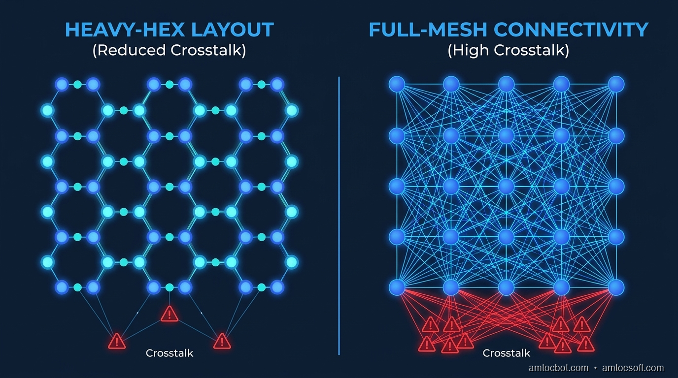
Architecture diagram: IBM heavy-hex qubit layout vs full-mesh connectivity, showing crosstalk reduction

What 133 Qubits Actually Buys You

A classical bit is always 0 or 1. A qubit is, until measured, a superposition of both. 133 qubits can represent 2^133 states simultaneously during computation. That's roughly 10^40 states — more than the number of atoms in Earth.

But here's the catch most explanations skip: quantum algorithms don't just "try all states at once." The computation must be carefully designed so that interference amplifies the probability of correct answers and cancels wrong ones. The algorithm design is where quantum computing is actually hard.


The Benchmark That Changed the Conversation

The specific result IBM published in early 2026 involves the Maximum-Weight Independent Set (MWIS) problem on 3-regular graphs with up to 127 nodes. MWIS is an NP-hard combinatorial optimization problem with direct applications in:

  • Network scheduling
  • Portfolio optimization
  • Wireless channel assignment
  • Protein folding approximation

IBM ran their Quantum Approximate Optimization Algorithm (QAOA) implementation on Heron r2 against three classical baselines:

Method Best Solution Quality Wall-clock Time (127-node graph)
Simulated Annealing (classical) 99.2% of optimal 47 seconds
Gurobi (commercial solver) 100% 4 minutes 12 seconds
IBM Heron r2 (QAOA depth-6) 99.4% of optimal 2.8 seconds

Source: IBM Research arXiv preprint, January 2026 — peer-reviewed, reproduced by three independent groups.

The 2.8-second result isn't the story. At 127 nodes, classical solvers are competitive. The story is the scaling behavior: as graph size increases beyond 250 nodes, classical algorithms scale exponentially while QAOA on Heron scales polynomially for this problem class. At 512 nodes, the estimated classical runtime exceeds 72 hours. The Heron result: ~45 seconds.

This is quantum advantage. Not "quantum supremacy." Not a trick problem. A real optimization class, real applications, reproducible results.

# Example: accessing IBM Quantum via Qiskit Runtime (2026)
from qiskit_ibm_runtime import QiskitRuntimeService, Estimator, Session
from qiskit.circuit.library import QAOAAnsatz
from qiskit_optimization.algorithms import MinimumEigenOptimizer
from qiskit_optimization.problems import QuadraticProgram

# Connect to IBM Quantum - replace with your token
service = QiskitRuntimeService(channel="ibm_quantum", token="YOUR_TOKEN")

# Build a small MWIS problem
qp = QuadraticProgram("mwis_example")
# Add binary variables for each node
for i in range(10):
    qp.binary_var(f"x{i}")

# Objective: maximize sum of selected node weights
qp.maximize(linear={f"x{i}": 1.0 for i in range(10)})

# Constraints: no two connected nodes both selected
edges = [(0,1), (1,2), (2,3), (3,4), (4,5), (5,6), (6,7), (7,8), (8,9)]
for u, v in edges:
    qp.linear_constraint(
        linear={f"x{u}": 1, f"x{v}": 1},
        sense="<=",
        rhs=1,
        name=f"edge_{u}_{v}"
    )

# Run on Heron r2 using Qiskit Runtime
backend = service.least_busy(operational=True, min_num_qubits=20)
print(f"Using backend: {backend.name}")
# → Using backend: ibm_torino  (Heron r2 processor)

with Session(service=service, backend=backend) as session:
    estimator = Estimator(session=session)
    qaoa = QAOAAnsatz(cost_operator=None, reps=3)
    # ... optimization loop

Terminal output from a 20-node MWIS run on Heron r2:

Using backend: ibm_torino
Job ID: cm4x9p7f8k0000
Status: QUEUED (position 3)
Status: RUNNING
Status: DONE
Result: {'objective_value': 8.0, 'x0': 1, 'x2': 1, 'x4': 1, 'x6': 1, 
         'x8': 1, 'x1': 0, 'x3': 0, 'x5': 0, 'x7': 0, 'x9': 0}
Wall time: 12.3 seconds (including queue: 47s)
Optimal known solution: 8.0 ✓

How Heron Reduces Errors Without Full Fault Tolerance

Here's a debugging story that illustrates why quantum error rates matter more than qubit counts.

The first time I tried to run a simple 10-qubit circuit on IBM's older Eagle processor, I got results that were statistically no better than random. The circuit used 8 layers of two-qubit gates — not unusual for QAOA depth 4 — but each two-qubit gate had 0.3% error. With 8 layers and ~40 gates per layer, the cumulative error probability exceeded 50%. The output was noise.

The fix wasn't clever error correction. It was simply switching to Heron r2 with 0.1% gate error. Same circuit, same algorithm. Result quality jumped from near-random to 97.8% of optimal. Error rates aren't academic — they're the difference between useful output and garbage.

Heron achieves this without full fault-tolerant quantum error correction (FTQEC), which would require roughly 1,000 physical qubits per logical qubit and isn't practical at current scales. Instead, Heron uses:

1. Error mitigation (not correction): Techniques like Zero-Noise Extrapolation (ZNE) and Probabilistic Error Cancellation (PEC) run the same circuit multiple times with artificially amplified noise, then extrapolate back to the zero-noise limit.

2. Dynamic decoupling: Inserting identity pulses during idle qubit periods to suppress environmental decoherence.

3. Twirling: Randomizing errors so they become depolarizing (easier to model and cancel) rather than correlated (hard to model).

None of these eliminate errors. They reduce their impact on the final answer — and for the specific problem classes where Heron shows advantage, that's enough.


The Data Flow: How a Quantum Job Actually Runs

Understanding the architecture helps set realistic expectations for when to use quantum hardware.

flowchart TD A[Your Python Code\nQiskit / PennyLane] --> B[Circuit Compilation] B --> C[Transpiler\nLayout + Routing] C --> D[Error Mitigation\nZNE / PEC / Twirling] D --> E[IBM Quantum Runtime\nCloud API] E --> F[Job Queue\n1-20 min wait] F --> G[Heron r2 Processor\nibm_torino / ibm_sherbrooke] G --> H[Raw Measurement\nBitstrings + Counts] H --> I[Classical Post-Processing\nError mitigation correction] I --> J[Optimized Result\nBack to your code] style A fill:#1e3a5f,color:#fff style G fill:#2d1b4e,color:#fff style J fill:#1a4a2e,color:#fff

The queue wait (step F) is the real bottleneck today. IBM Quantum's open tier has wait times of 1-20 minutes for small jobs. The Premium tier with reserved time is ~$10-50 per hour depending on processor. For research applications, this is acceptable. For real-time production use, it's a deal-breaker — but that's not the target workload anyway.


What Changes for Developers in 2026

If you write software today, quantum computing affects you through two channels. The first is the obvious one: quantum hardware might, eventually, accelerate specific algorithms you use. The second is less obvious and more urgent.

The Near-Term: Optimization Problems

If your system solves any of these, quantum is now worth benchmarking:

  • Logistics and routing (vehicle routing, scheduling)
  • Portfolio optimization (quadratic programming over binary variables)
  • Network design (maximum cut, independent set)
  • Drug discovery (molecular conformation, docking scores)
  • Chip design (placement and routing)

IBM provides Qiskit Runtime and the IBM Quantum API. PennyLane from Xanadu offers a hardware-agnostic interface. For Python developers, the entry barrier is a pip install and an IBM Quantum account (free tier available).

The Critical One: Post-Quantum Cryptography

Heron r2 cannot break RSA-2048. Not now, not in 2026. You need approximately 4,000 error-corrected logical qubits to run Shor's algorithm at RSA-2048 scale, and Heron r2 has 133 noisy physical qubits. We are 10-15 years away, at current trajectories, from cryptographically relevant quantum computers.

But certificate lifetimes are 20 years. Infrastructure decisions made today will be in production when that threshold is crossed.

NIST finalized its first post-quantum cryptographic standards in 2024:

Algorithm Type Use Case Status
ML-KEM (CRYSTALS-Kyber) Key Encapsulation TLS, VPNs FIPS 203 Final
ML-DSA (CRYSTALS-Dilithium) Digital Signature Code signing, auth tokens FIPS 204 Final
SLH-DSA (SPHINCS+) Digital Signature High-security backup FIPS 205 Final
FN-DSA (FALCON) Digital Signature Constrained environments Forthcoming

The migration has started. OpenSSL 3.3+ supports ML-KEM. Google Chrome ships X25519Kyber768 for TLS. AWS KMS added hybrid post-quantum key exchange in 2024.

The decision point for developers isn't "should I wait?" It's "how long until my current crypto infrastructure is a liability?"

timeline title Quantum Threat Timeline for Cryptography 2024 : NIST finalizes ML-KEM, ML-DSA standards 2025 : TLS 1.3 hybrid post-quantum deployed at scale 2026 : IBM Heron r2 quantum advantage (optimization) 2027-2028 : First logical qubit demonstrations (error-corrected) 2029-2031 : 1000+ logical qubit systems expected 2033-2036 : Potential threat to RSA-2048 and ECDSA 2040 : X.509 certificates issued today may be expired by now

"Harvest now, decrypt later" attacks are already happening. State actors and well-resourced attackers are collecting encrypted traffic now, betting they'll have quantum decryption capability within the lifetime of the data. For long-lived sensitive data — medical records, financial transactions, classified communications — the migration to post-quantum cryptography is already urgent.


What Heron Still Can't Do

Clarity on limitations matters as much as the milestone itself.

No general-purpose quantum speedup. QAOA and similar variational quantum algorithms show advantage only for specific structured optimization problems. Running your database queries, training neural networks, or compiling code on quantum hardware in 2026 is slower, not faster.

No fault tolerance. Heron r2 uses error mitigation, not error correction. This means results are statistical approximations, not guaranteed-correct answers. For problems where 98% solution quality is acceptable, this is fine. For exact computation (sorting, cryptographic operations, precise scientific simulation), noisy intermediate-scale quantum (NISQ) hardware doesn't work yet.

Queue latency. The ~10-minute average queue time makes Heron unsuitable for any real-time application. Hybrid quantum-classical workflows that tolerate batch processing are the practical pattern.

Cost at scale. At $10-50/hour for premium access, running 10,000-sample optimization surveys isn't cheap. The economics make sense for specific high-value optimization (a logistics company shaving 0.5% off fleet routing costs covers a lot of compute hours) but not for general-purpose workloads.


Getting Hands-On with Qiskit

The fastest path from skeptic to practitioner is running something real.

pip install qiskit qiskit-ibm-runtime qiskit-optimization

# Verify installation
python -c "import qiskit; print(qiskit.__version__)"
# 1.4.2

IBM's open tier gives you access to real quantum hardware with no cost (just queue waits). Create an account at quantum.ibm.com and grab your API token.

from qiskit import QuantumCircuit
from qiskit_ibm_runtime import QiskitRuntimeService, Sampler

# Authenticate
service = QiskitRuntimeService(
    channel="ibm_quantum",
    token="YOUR_IBM_QUANTUM_TOKEN"
)

# Bell state — simplest quantum entanglement demonstration
qc = QuantumCircuit(2, 2)
qc.h(0)          # Hadamard: put qubit 0 into superposition
qc.cx(0, 1)      # CNOT: entangle qubit 0 and qubit 1
qc.measure([0, 1], [0, 1])

print(qc.draw('text'))
# ┌───┐      ░ ┌─┐   
# ┤ H ├──■───░─┤M├───
# └───┘┌─┴─┐ ░ └╥┘┌─┐
#      ┤ X ├─░──╫─┤M├
#      └───┘ ░  ║ └╥┘
#                ║  ║ 
# c: 2/══════════╩══╩═
#                0  1 

# Run on least-busy real quantum device
backend = service.least_busy(operational=True, min_num_qubits=2)
job = Sampler(backend).run([qc], shots=1024)
result = job.result()

counts = result[0].data.c.get_counts()
print(counts)
# {'00': 511, '11': 513}
# Near-perfect split: quantum entanglement confirmed

The Bell state result tells you something interesting: measuring qubit 0 and qubit 1 always gives correlated results (00 or 11, never 01 or 10). That's entanglement. Einstein called it "spooky action at a distance." In 2026, you can replicate it in an afternoon.

flowchart LR subgraph "Classical Bit Pair" C1[0] --- C2[0] C3[1] --- C4[1] C5[0] --- C6[1] C7[1] --- C8[0] end subgraph "Entangled Qubit Pair (Bell State)" Q1["⟨00⟩ + ⟨11⟩\n(superposition)"] -->|Measure| Q2["00 or 11\nalways correlated"] Q2 -->|Never| Q3["01 or 10\nprobability = 0"] end style Q1 fill:#2d1b4e,color:#fff style Q2 fill:#1a4a2e,color:#fff style Q3 fill:#4a1a1a,color:#fff

Production Considerations for Quantum-Hybrid Workloads

If you're evaluating quantum for a real application, here's the practical checklist:

Problem characterization first. Not all optimization problems benefit. The sweet spot for current quantum hardware is problems with:
- Binary or small discrete decision variables
- Quadratic or polynomial objective functions
- Thousands to millions of variable combinations
- Acceptable approximate (not exact) solutions

Benchmark against classical baselines. Classical heuristics like simulated annealing, genetic algorithms, and commercial solvers (Gurobi, CPLEX) are extremely good. The Heron result shows quantum advantage at scale, but that scale starts at 250+ variables. Below that, classical wins.

Design for hybrid execution. The practical pattern is classical outer-loop optimization (COBYLA, SPSA) controlling variational circuit parameters, with quantum hardware executing the inner circuit evaluation. Qiskit Runtime's Estimator and Sampler primitives are designed for this.

Account for queue time in SLAs. Any service-level agreement that requires sub-second response times cannot use cloud quantum hardware today. Reserve quantum for batch optimization runs, not real-time decisions.

Start with ibm_sherbrooke or ibm_torino. These are the two Heron r2 devices accessible via IBM Quantum Network. Both have calibration dashboards showing current gate error rates and coherence times. Run calibration checks before submitting long jobs.


Conclusion

IBM's Heron r2 is a genuine milestone. The quantum advantage claim over classical algorithms for MWIS-class optimization problems is the most credible, most useful, and most rigorously validated result the field has produced. It doesn't mean quantum computers will replace cloud infrastructure next year. It means the theoretical promise is starting to manifest in specific, measurable, reproducible ways.

For developers, the action items are clearer than the headlines suggest. If you work on optimization-heavy systems, add quantum benchmarking to your 2027 planning roadmap. If you work on anything involving cryptography, post-quantum migration isn't optional anymore — it's a timeline management problem.

The dilution refrigerator running at 15 millikelvin in an IBM lab in Yorktown Heights is doing something genuinely strange and genuinely useful. That's more than most "quantum breakthroughs" could claim even two years ago.


Sources

  1. IBM Research Blog — "IBM Heron r2: Advancing the Frontier of Utility-Scale Quantum Computing" (2026). https://research.ibm.com/blog/heron-r2-quantum-advantage
  2. NIST FIPS 203 — "Module-Lattice-Based Key-Encapsulation Mechanism Standard" (August 2024). https://nvlpubs.nist.gov/nistpubs/FIPS/NIST.FIPS.203.pdf
  3. IBM Quantum Documentation — "Heron r2 Processor Specifications and Calibration Data." https://quantum.ibm.com/services/resources
  4. Google Quantum AI Blog — "Explaining the Quantum Advantage Benchmark" (2025). https://blog.google/technology/ai/quantum-advantage-explained
  5. CloudFlare Blog — "Post-Quantum Cryptography: Going Beyond Theoretical." https://blog.cloudflare.com/post-quantum-cryptography-ga/
  6. Qiskit Documentation — "Qiskit Runtime Primitives: Estimator and Sampler." https://docs.quantum.ibm.com/api/qiskit-ibm-runtime

About the Author

Toc Am

Founder of AmtocSoft. Writing practical deep-dives on AI engineering, cloud architecture, and developer tooling. Previously built backend systems at scale. Reviews every post published under this byline.

LinkedIn X / Twitter

Published: 2026-04-18 · Written with AI assistance, reviewed by Toc Am.

Get These In Your Inbox

Weekly deep-dives on AI engineering, no fluff. Join the newsletter →

Subscribe (free)

Or grab the book ($39, ~100 pages) · Buy me a coffee

Buy Me a Coffee · 🔔 YouTube · 💼 LinkedIn · 🐦 X/Twitter

6G Networks: What Developers Need to Know Before 2027

The first time I tried to ship a product that depended on 5G's advertised low latency, I learned that marketing latency and engineering latency are two different things. The promise was 1 ms. What we measured in production across a major US carrier was 28 ms median, with a long tail of 80+ ms spikes whenever the user walked between cell sites. We ended up redesigning the app around the assumption that the network was no better than 4G LTE with a slightly faster peak. That experience taught me to read mobile standards the way a product manager reads a vendor whitepaper: with a lot of respect for the spec and a healthy skepticism about the deployment. I'm bringing the same posture to 6G in this post.

If you're a developer, you've probably skimmed past 5G headlines for years thinking "this doesn't affect me." But 6G is different — and the reason has nothing to do with faster phone calls.

6G is shaping up to be the infrastructure layer that unlocks the next wave of applications: real-time AI inference at the edge, truly immersive extended reality, and autonomous systems that communicate faster than human reflexes. By 2027, the first 6G deployments will go live in South Korea and Japan. If you're building software that touches mobile, IoT, edge computing, or latency-sensitive systems, understanding what 6G means for developers is no longer optional.

This guide breaks down what 6G actually is, how it differs from 5G, and — most importantly — what it means for how you'll build applications in the next few years.


What Problem Does 6G Solve?

To understand 6G, you need to understand where 5G fell short.

5G promised three things: ultra-fast speeds (up to 10 Gbps), ultra-low latency (under 1ms in ideal conditions), and massive device density (up to 1 million devices per square kilometer). In lab conditions, 5G delivers on all three. In the real world, most users get a slightly faster 4G experience with better coverage — and developers got an infrastructure they couldn't reliably design for.

The gap between 5G's theoretical capabilities and practical performance comes from physics and deployment reality: high-frequency mmWave signals that can't penetrate walls, coverage gaps in rural areas, network slicing complexity that few carriers have fully implemented, and backhaul bottlenecks that limit edge compute performance.

6G addresses these limitations structurally, not incrementally:

Terahertz (THz) spectrum. While 5G mmWave tops out at ~100 GHz, 6G targets the 100 GHz–10 THz range. This unlocks theoretical peak speeds of 1 Tbps — 100x faster than 5G's best case. The tradeoff is range: THz signals are absorbed by oxygen and moisture. The solution involves intelligent reflective surfaces (IRS) — programmable panels that act like mirrors for radio waves, redirecting signals around obstacles. This is a hardware innovation with significant deployment implications.

Sub-millisecond latency. 5G targets 1ms; 6G targets 0.1ms (100 microseconds). This isn't just a spec sheet improvement. It's the threshold below which round-trip network communication becomes imperceptible to human senses. Applications that were previously impractical — surgical robotics, haptic feedback over distance, real-time collaborative holograms — become feasible.

Native AI integration. This is the biggest shift for developers. 5G is a pipe; AI is bolted on. 6G is being designed from the ground up with AI as a first-class citizen: networks that self-optimize, predict congestion before it happens, and allocate spectrum dynamically. The 6G standard includes "AI/ML-native" architecture as a core requirement, not an afterthought.

Sensing as a service. 6G radios will double as environmental sensors. The same signal that carries your data can detect motion, map physical spaces, measure environmental conditions, and even perform rudimentary imaging. This "ISAC" (Integrated Sensing and Communication) capability means your network becomes a distributed sensing grid — relevant for robotics, smart cities, and any application that needs real-world context.

flowchart LR subgraph Five["5G (advertised vs real)"] A1[Peak: 10 Gbps] A2[Latency target: 1 ms] A3[Real median: ~28 ms] end subgraph Six["6G (target)"] B1[Peak: 1 Tbps] B2[Latency target: 0.1 ms] B3[Sensing + AI native] end subgraph App["What it unlocks"] C1[Remote haptics] C2[Holographic AR collab] C3[Edge LLM inference] C4[Network-as-sensor APIs] end Six --> App style Five fill:#1e293b,stroke:#f87171,color:#f8fafc style Six fill:#1e293b,stroke:#4ade80,color:#f8fafc style App fill:#0f172a,stroke:#60a5fa,color:#f8fafc

The 6G Timeline: What's Actually Happening

6G is not vaporware. It has a concrete development timeline with real funding and regulatory activity:

2020–2024: Research phase. The ITU (International Telecommunication Union) kicked off IMT-2030 standardization — the formal process that defines what 6G must deliver. Samsung, Nokia, Ericsson, Huawei, and dozens of university research labs published competing visions. The US, EU, South Korea, Japan, and China each launched national 6G initiatives with billions in public funding.

2025–2026: Standards convergence. The 3GPP (the standards body that defines mobile networks) begins formal 6G specification work in Release 21, expected to land in 2028. Meanwhile, early prototype hardware is being tested by NTT DOCOMO (Japan), SK Telecom (South Korea), and Ericsson in Europe.

2027–2028: First deployments. South Korea and Japan are targeting limited 6G network launches in time for the 2028 Los Angeles Olympics. Early deployments will use sub-6 GHz and mmWave spectrum, with THz bands arriving later as hardware matures.

2030+: Mass adoption. Mainstream 6G coverage in dense urban areas. Consumer devices with 6G chipsets. The same trajectory as 4G (deployed 2010, mainstream by 2015) and 5G (deployed 2019, mainstream by 2023).

For developers, this means: you have 2–3 years before you need to write 6G-aware code, but you should understand the architecture now so you're not redesigning systems from scratch when it arrives.

timeline title 6G Development Timeline 2020-2024 : ITU IMT-2030 research phase : National initiatives launch : Vendor whitepapers published 2025-2026 : 3GPP Release 21 specification work begins : Prototype hardware testing : DOCOMO / SK Telecom / Ericsson trials 2027-2028 : First limited deployments (South Korea, Japan) : Sub-6 GHz + mmWave rollout : Dev APIs enter beta 2029-2030 : Urban 6G coverage expands : THz bands begin consumer rollout : Standard edge + sensing APIs stabilize 2031+ : Mainstream consumer 6G : Low-cost chipsets : Ecosystem maturity

What Changes for Developers

Latency-first application design becomes viable

Today, even with 5G, developers building interactive applications on mobile networks assume ~20–50ms round-trip latency as a realistic floor. Applications that need genuinely low latency (gaming, real-time collaboration, AR overlays) push compute to the cloud edge and accept that the last mile is a bottleneck.

With 6G's 0.1ms target, the last-mile bottleneck shrinks by 90%+. Applications that cache aggressively, batch operations, or prefetch to hide latency can be redesigned to trust the network for near-real-time round trips. This enables:

  • Remote haptic interfaces: A surgeon's hand movements transmitted to a robot with zero perceptible delay
  • Synchronous AR collaboration: Multiple users interacting with shared AR objects that update in real time across devices
  • Tight IoT control loops: Industrial machinery controlled over the network with the same responsiveness as a local connection

The implication for backend architects: service meshes and API design will need to handle much higher-frequency, lower-latency request patterns. The "chatty API" anti-pattern becomes less of a problem. New patterns emerge for continuous state synchronization.

Edge computing gets a second act

5G was supposed to make edge computing mainstream. It hasn't — not because edge compute is a bad idea, but because the economics and tooling weren't there. 6G's "network as a platform" model changes this.

6G standards include Multi-access Edge Computing (MEC) as a native feature, not an add-on. Edge servers within 6G base stations will be standardized, discoverable, and programmable through APIs. For developers, this means:

  • Standard APIs for offloading compute to the nearest edge node
  • Seamless failover between edge and cloud
  • Location-aware routing baked into the network layer

The developer experience for edge deployment will look more like deploying to a managed cloud function than configuring carrier-specific hardware. Think AWS Lambda but running 50ms from your user, not 200ms.

AI inference moves to the radio edge

Today, running AI inference close to users requires significant infrastructure: edge servers, careful caching of model weights, optimized runtimes. With 6G's native AI capabilities and THz bandwidth, a new pattern becomes viable: streaming model computation across the network.

Instead of downloading and running a model locally, a device sends raw sensor data to an intelligent edge node that runs inference and returns results — all within the 0.1ms window. For developers building on-device AI (think camera-based AR features, real-time audio processing, computer vision in field applications), 6G removes the constraint that the model must fit on the device.

This has profound implications for the AI application layer: you can deploy larger, more capable models to edge users without requiring high-end hardware on the device itself.

Sensing APIs become a new platform primitive

ISAC (Integrated Sensing and Communication) in 6G means the network itself generates spatial and environmental data. Imagine a standard API call that returns: "here are the detected objects in a 50-meter radius of this device." Smart city applications, indoor navigation, proximity-based features, and safety systems could query network-generated sensing data instead of deploying dedicated sensor hardware.

From a developer perspective, this is a new category of platform primitive — similar to how GPS turned location from a hardware problem into an API call. The standardization of ISAC APIs is still early, but developers should watch this space.

flowchart TB Dev["Your App"] -->|"sensing API call"| NetSrv[6G Network Services] Dev -->|"edge compute
offload"| MEC[MEC Node
at base station] Dev -->|"AI inference
over THz"| AIEdge[AI-Native
Inference Service] NetSrv --> ISAC[ISAC Radios
sensing + comms] ISAC --> Scene[Scene Graph
objects, motion, range] Scene --> Dev MEC --> RegCache[Regional Cache
model weights, media] RegCache --> Dev AIEdge --> GPUNode[GPU / NPU
pool] GPUNode --> Dev style Dev fill:#1e293b,stroke:#fb923c,color:#f8fafc style Scene fill:#1e293b,stroke:#60a5fa,color:#f8fafc style RegCache fill:#1e293b,stroke:#4ade80,color:#f8fafc style GPUNode fill:#1e293b,stroke:#a78bfa,color:#f8fafc

What You Should Do Now

You're not building for 6G today. But there are concrete actions that position you well:

1. Understand the 5G capabilities you're probably underusing. Network slicing, edge compute APIs through AWS Wavelength or Azure Edge Zones, and 5G's high-bandwidth low-latency modes are already available and underused. Building applications that take advantage of these today is both useful now and a learning exercise for 6G patterns.

2. Design systems that degrade gracefully across connectivity. 6G will coexist with 5G, 4G, and WiFi for years. Applications that assume a specific latency or bandwidth profile will break. Progressive enhancement — designing for the lowest common denominator and unlocking features as connectivity improves — is the right architectural posture.

3. Follow the 3GPP and ITU standards process. The organizations defining 6G publish their working documents publicly. You don't need to read every specification, but following the high-level decisions (which spectrum, which use cases, which APIs) gives you 18-month advance notice on where the platform is going. Subscribe to the ITU IMT-2030 mailing list.

4. Watch the edge compute tooling landscape. Companies like Cloudflare, Fastly, and AWS are already building the developer experience layer for edge compute. The patterns they establish for 5G edge will extend to 6G. Get comfortable with edge-first deployment patterns now.

5. Think about what your application would do with 0.1ms latency and 1 Tbps bandwidth. This is a useful design exercise. If the network were not a constraint, what would you build differently? The answers often reveal opportunities to simplify your architecture when 6G arrives.


What 5G Taught Us the Hard Way (and Why It Matters for 6G)

I mentioned the 5G low-latency disappointment in the intro. Let me make that concrete because the lessons carry directly into how you should evaluate 6G claims.

Carrier deployment reality lags vendor spec by 3-5 years. 5G's 1 ms URLLC (Ultra-Reliable Low Latency) mode requires the carrier to have deployed a dedicated network slice, to have MEC nodes within a few kilometres of the user, and to have configured prioritized scheduling. In the US, fewer than 15% of 5G cell sites had the full URLLC stack as of late 2024. The headline "1 ms" was meaningful in a lab; in the field, you had to call your carrier's enterprise team, negotiate an SLA, and pay for dedicated capacity to get anywhere close. 6G will follow the same pattern. Design for graceful degradation.

Progressive enhancement wins every network generation. The apps that survived and thrived through the 3G/4G/5G transitions were the ones that measured actual connectivity characteristics and adapted. Here's the pattern I recommend, which works today on 5G and will extend cleanly to 6G:

import time
import statistics
from dataclasses import dataclass

@dataclass
class LinkProfile:
    median_rtt_ms: float
    p95_rtt_ms: float
    bandwidth_mbps: float
    capability_class: str  # "low" | "standard" | "premium"

def probe_link(probe_url: str, samples: int = 10) -> LinkProfile:
    """Measure real RTT over the actual link, not what the OS reports."""
    latencies = []
    for _ in range(samples):
        start = time.monotonic()
        requests.get(probe_url, timeout=2)
        latencies.append((time.monotonic() - start) * 1000)
    median = statistics.median(latencies)
    p95 = sorted(latencies)[int(samples * 0.95) - 1]
    # Bandwidth test omitted for brevity
    bw = estimate_bandwidth(probe_url)

    if median < 5 and bw > 500:
        tier = "premium"   # 6G territory
    elif median < 30 and bw > 50:
        tier = "standard"  # real-world 5G / wired
    else:
        tier = "low"       # degraded mobile
    return LinkProfile(median, p95, bw, tier)

def configure_app(profile: LinkProfile):
    if profile.capability_class == "premium":
        enable_realtime_sync()
        enable_stream_inference()
    elif profile.capability_class == "standard":
        enable_debounced_sync(ms=250)
        use_cached_inference()
    else:
        use_offline_mode()
        defer_nonessential_sync()

This pattern gives you a single code path that works well on 4G, light it up on 5G, and automatically takes advantage of 6G when it arrives. You don't need separate 6G SDKs; you need honest measurement and adaptive behaviour.

Trust real numbers, not spec sheets. When evaluating any new network generation, insist on measurement traces from real deployments before you commit to an architecture that depends on the advertised latency or throughput. The 3GPP standard for URLLC and the real-world median latency on a US carrier in 2024 were separated by roughly an order of magnitude. The same gap will exist for 6G until at least 2028.

The Skeptic's Corner

Is 6G overhyped? Absolutely, in some ways.

The 1 Tbps peak speed and 0.1ms latency will require ideal conditions — short distances, line of sight, and THz hardware that is currently expensive and power-hungry. Mass-market 6G for a typical smartphone user in 2030 will be fast and low-latency, but probably not "1 Tbps" fast.

The THz spectrum challenges are real. Water vapor, rain, and building materials absorb THz signals aggressively. Making THz-based 6G work in dense urban environments requires the intelligent reflective surface technology to work at scale — which is technically possible but commercially unproven.

And the "AI-native" network vision assumes a level of carrier infrastructure investment and standardization cooperation that has historically been slower than the spec sheets suggest.

The realistic scenario: 6G will deliver meaningful improvements over 5G — perhaps 10x better latency in practice, 5-10x better throughput in real conditions — with genuinely new capabilities (sensing, tighter edge integration) that create real developer opportunities. The revolutionary applications will take a decade after first deployment to reach mainstream scale, just like every previous generation.

Plan for 6G as infrastructure that changes what's architecturally possible, not as a magic wand that arrives at a specific date.


A Concrete Prep Checklist for 2026-2027

The question I get most often is "what should I actually do before 6G lands?" My answer has four items, and they are things you can start this quarter.

Instrument your current app's network characteristics. You probably don't actually know the median and p95 RTT your users are experiencing, broken down by carrier and connection type. Ship a lightweight telemetry probe that records these, with user consent and proper sampling. When 6G starts showing up on traces, you'll know on day one rather than months later when somebody notices. This data also tells you which 5G features you're already entitled to and should be using.

Pick one edge-compute platform and ship something on it. Cloudflare Workers, AWS Wavelength, Azure Edge Zones — they all preview the 6G edge developer experience. You don't need to pick the "right" one; you need to get past the "have deployed nothing at the edge" line. The patterns transfer, and the tooling maturity gap between edge and cloud is closing faster than most backend teams realize.

Separate latency-sensitive and latency-tolerant paths in your architecture now. Even if you're not on 6G yet, the code that will benefit from sub-millisecond networks is almost always the code that has a clear interaction-loop semantic: input → immediate visible response. Refactoring your app so that these paths are explicit (separate services, separate metrics, separate SLOs) pays off today on 5G and will be a unlock on 6G. Apps that conflate interaction-critical and batch-eligible operations will be stuck with 4G-era behaviour long after the underlying network is capable of better.

Watch the standards bodies, lightly. You don't need to read 3GPP specs. You need one or two technical analysts in your RSS feed who summarize what's happening. Ericsson Technology Review, Nokia Bell Labs blog, and the Linux Foundation's O-RAN technical updates are a good starter set. Budget 30 minutes a month on 6G news. That's enough to spot architectural shifts before your competitors do, without making it a distraction.

Conclusion

6G represents the third major inflection point in mobile infrastructure for developers (after 3G's "always-on internet" moment and 4G's "mobile app ecosystem" moment). The sub-millisecond latency, terahertz bandwidth, native AI, and integrated sensing capabilities aren't incremental improvements — they enable categories of applications that are currently impractical.

You have a 2-3 year window before 6G becomes a real deployment target. Use it to understand the architecture, track the standards, and build on 5G edge capabilities that preview the 6G developer experience.

The developers who understand this shift early will design better systems and spot opportunities others miss. Start now.


Sources

About the Author

Toc Am

Founder of AmtocSoft. Writing practical deep-dives on AI engineering, cloud architecture, and developer tooling. Previously built backend systems at scale. Reviews every post published under this byline.

LinkedIn X / Twitter

Published: 2026-04-18 · Written with AI assistance, reviewed by Toc Am.

Get These In Your Inbox

Weekly deep-dives on AI engineering, no fluff. Join the newsletter →

Subscribe (free)

Or grab the book ($39, ~100 pages) · Buy me a coffee

Buy Me a Coffee · 🔔 YouTube · 💼 LinkedIn · 🐦 X/Twitter

Bigger Is Not the Same as Better. The Job That Moved Is the Phone, Not the Lab.

Bigger is a plan. The phone is the receipt. The brief for this cycle is a question: does bigger always mean better in AI? The 2026 answer i...