Showing posts with label Advanced. Show all posts

Monday, April 6, 2026

Fine-Tuning vs RAG: When to Use Which

Fine-Tuning vs RAG Hero

Level: Advanced | Topic: Fine-Tuning vs RAG | Read Time: 7 min

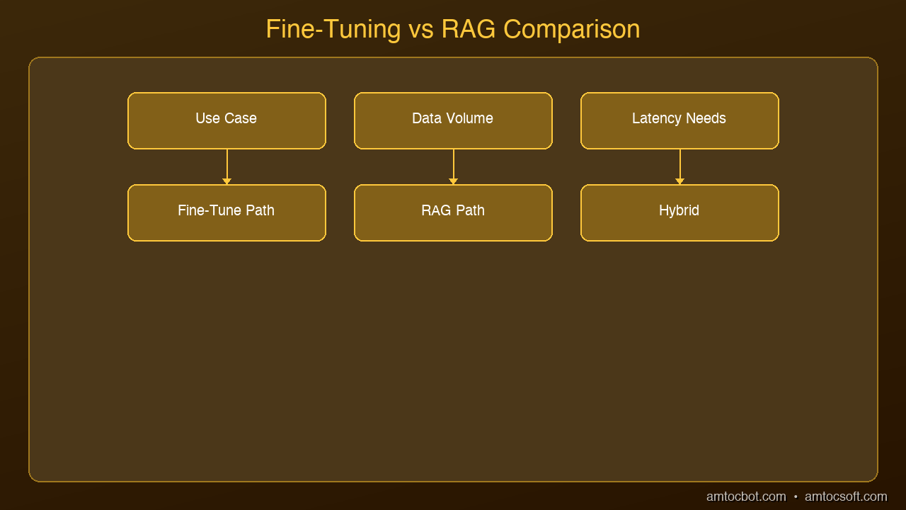
Two techniques dominate the conversation about customizing LLMs: fine-tuning and Retrieval-Augmented Generation (RAG). Both make models more useful for specific tasks. But they solve fundamentally different problems, and using the wrong one wastes time and money.

This guide provides a clear decision framework for choosing between them.

Animated flow diagram

What Each Technique Does

RAG adds external knowledge at inference time. Before the model generates a response, RAG searches a knowledge base, retrieves relevant documents, and includes them in the prompt. The model's weights remain unchanged.

Fine-tuning changes the model's behavior by updating its weights with new training data. The model permanently learns new patterns, styles, or domain knowledge.

The distinction matters: RAG teaches the model what to know. Fine-tuning teaches the model how to behave.

When to Use RAG

Architecture Diagram

RAG is the right choice when:

  • Knowledge changes frequently: Product catalogs, documentation, news, pricing — anything that updates regularly
  • You need citations: RAG naturally provides source documents for every answer
  • Your knowledge base is large: RAG can search millions of documents without increasing model size
  • Accuracy is critical: Grounding responses in retrieved documents reduces hallucinations
  • You need to get started quickly: RAG requires no training, just a vector database and embeddings

Common RAG use cases: customer support chatbots, document Q&A, knowledge base search, legal research, internal wikis.

When to Use Fine-Tuning

Fine-tuning is the right choice when:

  • You need a specific output format: Always return JSON, always use a template, always follow a rubric
  • You need a specific tone or style: Brand voice, medical writing style, legal prose
  • You need improved reasoning in a domain: Medical diagnosis, code review, financial analysis
  • Latency matters: Fine-tuned models respond in one pass; RAG adds retrieval latency
  • You want a smaller, faster model: Fine-tune a 3B model to outperform a general 70B on your task

Common fine-tuning use cases: code generation for specific frameworks, clinical note summarization, sentiment analysis in a specific domain, structured data extraction.

The Decision Matrix

| Criterion | Choose RAG | Choose Fine-Tuning |

|-----------|-----------|-------------------|

| Knowledge freshness | Dynamic, changes often | Static domain knowledge |

| Training data available | Not enough examples | 1,000+ quality examples |

| Output format needs | Standard text | Specific structure required |

| Deployment speed | Need it now | Can invest training time |

| Cost sensitivity | Low ongoing cost | Upfront training cost |

| Model behavior change | No | Yes |

The Best Answer: Use Both

The most effective production systems combine both techniques:

1. Fine-tune the base model on your domain to improve its reasoning and output format

2. Add RAG to give it access to current knowledge and specific documents

3. Engineer prompts to guide the fine-tuned model's behavior at inference time

Example: A medical AI that is fine-tuned on clinical notes (behavior), uses RAG to retrieve patient records (knowledge), and has a system prompt defining the output template (format).

Cost Comparison

| Approach | Upfront Cost | Ongoing Cost | Maintenance |

|----------|-------------|-------------|-------------|

| RAG only | Vector DB setup | Embedding + retrieval per query | Update documents |

| Fine-tuning only | GPU training time | Inference compute | Retrain periodically |

| Both | Higher initial | Moderate | Both maintenance streams |

For most teams, starting with RAG and adding fine-tuning when needed is the pragmatic path.

Sources & References:

1. Lewis et al. — "Retrieval-Augmented Generation" (2020) — https://arxiv.org/abs/2005.11401

2. Hu et al. — "LoRA: Low-Rank Adaptation" (2021) — https://arxiv.org/abs/2106.09685

3. LangChain — "RAG Documentation" — https://python.langchain.com/docs/concepts/rag/

*Published by AmtocSoft | amtocsoft.blogspot.com*

*Level: Advanced | Topic: Fine-Tuning vs RAG*


Enjoyed this post? Follow AmtocSoft for AI tutorials from beginner to professional.

Buy Me a Coffee | 🔔 YouTube | 💼 LinkedIn | 🐦 X/Twitter

LoRA and QLoRA Explained: Fine-Tuning AI on a Budget

LoRA and QLoRA Explained Hero

Level: Advanced | Topic: Fine-Tuning | Read Time: 8 min

Traditional fine-tuning updates every parameter in a model. For a 7-billion parameter model, that means storing and updating 7 billion floating-point numbers. This requires multiple high-end GPUs and significant memory.

LoRA changed that. Low-Rank Adaptation is a technique that makes fine-tuning accessible to anyone with a single consumer GPU. QLoRA takes it further by adding quantization to the mix.

This article explains both techniques and shows why they have become the default approach for fine-tuning open-source models.

Animated flow diagram

The Problem with Full Fine-Tuning

A 7B parameter model in float16 requires approximately 14 GB of GPU memory just to store the weights. During training, you also need memory for gradients and optimizer states, which typically triples the requirement to 42+ GB. That exceeds the capacity of most consumer GPUs.

For a 70B parameter model, full fine-tuning requires a cluster of A100 GPUs. For most developers and organizations, this is prohibitively expensive.

LoRA: The Key Insight

Architecture Diagram

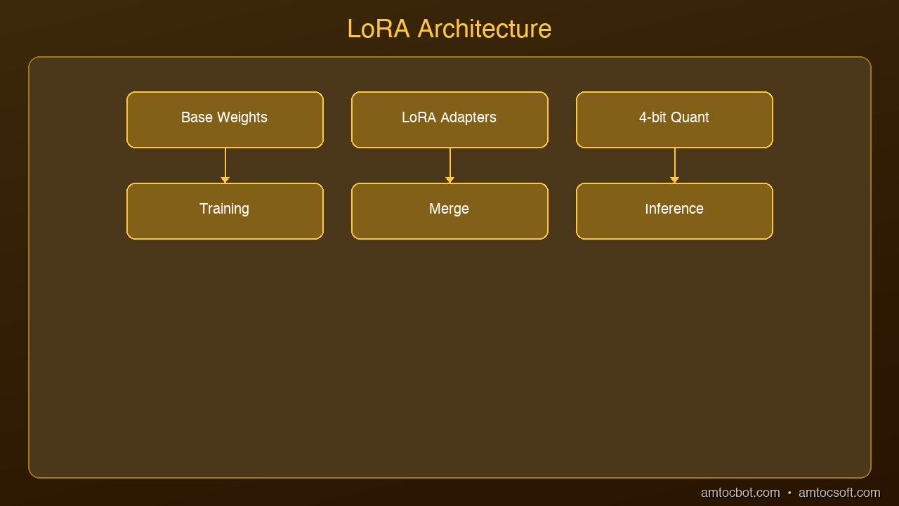
LoRA is based on a simple but powerful observation: when you fine-tune a large language model, the weight updates tend to be low-rank. In other words, the changes can be approximated by much smaller matrices.

Instead of updating the full weight matrix W (which might be 4096 x 4096), LoRA freezes the original weights and trains two small matrices A and B:

  • A: 4096 x r (where r is typically 8, 16, or 32)
  • B: r x 4096

The effective update is the product A x B, which has the same dimensions as W but is parameterized by far fewer numbers. For rank r=16, you are training 131,072 parameters instead of 16,777,216. That is a 128x reduction.

What This Means in Practice

| Metric | Full Fine-Tuning | LoRA (r=16) |

|--------|-----------------|-------------|

| Trainable parameters | 7B (100%) | ~55M (0.8%) |

| GPU memory required | 42+ GB | 8-12 GB |

| Training time (7B) | Hours on A100 cluster | 30-60 min on single GPU |

| Storage per adapter | 14 GB | 50-200 MB |

| Quality | Baseline | 95-99% of full fine-tuning |

The quality trade-off is remarkably small. Research consistently shows LoRA achieving within a few percentage points of full fine-tuning on most benchmarks.

QLoRA: Adding Quantization

QLoRA combines LoRA with 4-bit quantization of the base model. Instead of loading the frozen weights in float16 (2 bytes per parameter), QLoRA loads them in 4-bit precision (0.5 bytes per parameter).

This reduces the memory footprint by another 4x. A 7B model that requires 14 GB in float16 needs only 3.5 GB in 4-bit quantization. Combined with LoRA's small adapter matrices, you can fine-tune a 7B model on a GPU with 6 GB of VRAM.

The key innovation is that QLoRA uses a technique called NormalFloat4 (NF4), which is information-theoretically optimal for normally distributed weights. Combined with double quantization (quantizing the quantization constants), it achieves quality nearly identical to float16 LoRA.

When to Use LoRA vs QLoRA

Use LoRA when: You have a GPU with 12+ GB VRAM and want the highest quality fine-tuning with minimal trade-offs.

Use QLoRA when: You have a consumer GPU (6-8 GB VRAM) and need to fine-tune within memory constraints. Or when fine-tuning larger models (13B, 70B) on limited hardware.

Use full fine-tuning when: You have enterprise GPU resources and need absolute maximum quality, or you are training a model from scratch.

Tools for LoRA Fine-Tuning

The ecosystem has matured rapidly:

  • Unsloth: Fastest LoRA training, 2-5x speedup over standard implementations
  • Hugging Face PEFT: The reference implementation, integrates with all HF models
  • Axolotl: Simplified config-driven fine-tuning with LoRA/QLoRA support
  • LLaMA-Factory: GUI-based fine-tuning with dozens of model templates

Practical Tips

1. Start with rank r=16. Increase to 32 or 64 only if quality is insufficient.

2. Apply LoRA to all linear layers, not just attention. Recent research shows this improves quality.

3. Use a learning rate of 1e-4 to 3e-4. LoRA is less sensitive to learning rate than full fine-tuning.

4. Train for 1-3 epochs. More epochs risk overfitting on small datasets.

5. Use at least 1,000 high-quality training examples. Quality matters more than quantity.

Sources & References:

1. Hu et al. — "LoRA: Low-Rank Adaptation of Large Language Models" (2021) — https://arxiv.org/abs/2106.09685

2. Dettmers et al. — "QLoRA: Efficient Finetuning of Quantized Language Models" (2023) — https://arxiv.org/abs/2305.14314

3. Hugging Face — "PEFT: Parameter-Efficient Fine-Tuning" — https://huggingface.co/docs/peft

*Published by AmtocSoft | amtocsoft.blogspot.com*

*Level: Advanced | Topic: Fine-Tuning, LoRA*


Enjoyed this post? Follow AmtocSoft for AI tutorials from beginner to professional.

Buy Me a Coffee | 🔔 YouTube | 💼 LinkedIn | 🐦 X/Twitter

Voice Agent Architectures: Pipelines vs End-to-End Models

Level: Advanced

Topic: Voice AI, TTS, STT

Hero Image: Two diverging paths -- pipeline components vs single end-to-end model

If you've built a voice agent using the pipeline approach from our previous tutorial -- STT into LLM into TTS -- you've already seen it work. But you've probably also noticed the latency. Every stage adds time, and the stages are sequential. The industry median for voice agent response time is 1.4-1.7 seconds -- five times slower than the 300ms natural pause in human conversation.

Is there a better way?

In 2026, three competing architectural paradigms are battling for dominance: the cascading pipeline (what we built), the end-to-end speech-to-speech model (what OpenAI and Google are pushing), and the managed platform (what Retell, VAPI, and Bland are selling). Each has profound trade-offs in latency, flexibility, cost, and capability.

This post goes deep on all three, compares the major platforms with real pricing and performance data, and helps you choose the right architecture for your use case.

Architecture 1: The Cascading Pipeline

The pipeline approach chains three independent models together:

Animated flow diagram

How It Works

1. Raw audio from the microphone flows into the STT engine

2. STT produces a text transcription

3. The text goes to an LLM as a user message

4. The LLM generates a text response (with optional function calling)

5. The text response goes to a TTS engine

6. TTS produces audio that plays through the speaker

Each component is independent, replaceable, and debuggable.

Latency Breakdown (Production Reality)

Every stage adds latency. Here's a realistic breakdown based on production systems:

User finishes speaking
  |
  +-- VAD end-of-speech detect:     50ms     (P50)  /  100ms  (P99)
  |
  +-- STT finalization:            100ms     (P50)  /  250ms  (P99)
  |
  +-- Network to LLM:              10ms     (P50)  /   30ms  (P99)
  |
  +-- LLM time-to-first-token:    150ms     (P50)  /  400ms  (P99)
  |     (accounts for 70% of total latency)
  |
  +-- Network to TTS:              10ms     (P50)  /   30ms  (P99)
  |
  +-- TTS time-to-first-byte:     100ms     (P50)  /  250ms  (P99)
  |
  +-- Audio buffer + playback:     50ms     (P50)  /  100ms  (P99)
  |
  = Total:                        470ms     (P50)  / 1160ms  (P99)

The LLM is the bottleneck. It accounts for roughly 70% of total latency. This is why swapping GPT-4o-mini for GPT-4o can shave 100-200ms off every response.

Streaming Optimization

The key to making pipelines fast is streaming overlap -- don't wait for one stage to finish before starting the next:

1. Start LLM inference as soon as STT produces a final transcript

2. Start TTS as soon as the LLM produces the first sentence (not the full response)

3. Start audio playback as soon as TTS produces the first audio chunk

4. Keep persistent API connections to eliminate handshake latency

With full streaming optimization, a pipeline can hit 400-600ms P50 consistently -- acceptable for most conversational use cases.

Advantages

  • Flexibility: Swap any component independently. Don't like ElevenLabs? Switch to Kokoro. Want Claude instead of GPT-4o? Change one line of code.
  • Debuggability: Inspect text between stages. Log every transcript, every LLM response, every TTS input. When something goes wrong, you know exactly which stage failed.
  • Best-of-breed: Use the best STT (Deepgram for streaming), the best LLM (GPT-4o for reasoning), and the best TTS (ElevenLabs for quality) -- they don't have to come from the same vendor.
  • Text-based tools: The LLM operates on text, so all existing function-calling, RAG, and prompt engineering techniques work without modification.
  • Cost control: Price each component independently. Use a cheap LLM for simple queries, expensive one for complex ones.

Disadvantages

  • Cumulative latency: Three serial stages = three sets of latency stacked
  • Lost audio information: STT converts speech to text, losing tone, emotion, hesitation, emphasis. The LLM never hears *how* you said something.
  • Error propagation: STT mistakes cascade. "I need to book a flight" transcribed as "I need to cook a flight" gives the LLM garbage input.
  • Turn-taking complexity: Detecting when the user has finished speaking requires separate VAD tuning.

Open-Source Pipeline Frameworks

Pipecat (~1,872 GitHub stars):

  • Created by Daily.co, Python-only
  • 60+ provider integrations (the most of any framework)
  • Client SDKs: JavaScript, React, React Native, iOS, Android, C++
  • Pipecat Cloud for managed hosting
  • Best for: Teams wanting maximum provider flexibility

LiveKit Agents (~9,900 GitHub stars):

  • Open-source WebRTC platform + agent framework
  • Python and Node.js SDKs
  • Semantic turn detection (transformer-based, more sophisticated than VAD alone)
  • Multi-agent handoff, MCP support
  • Agent Builder for no-code prototyping
  • Best for: Teams already using LiveKit, or wanting WebRTC infrastructure

Vocode (open-source, community-maintained):

  • Python library + enterprise API
  • Looking for community maintainers (signal of reduced commercial investment)
  • Zoom integration
  • Best for: Simple use cases, Zoom-focused deployments

Architecture 2: End-to-End Speech-to-Speech Models

End-to-end models process audio directly -- no separate STT/TTS stages. The model receives audio waveforms as input and produces audio waveforms as output.

Animated flow diagram

How It Works

Instead of converting audio to text and back, an end-to-end model:

1. Encodes the input audio into a latent representation

2. Processes that representation through a language model that understands audio natively

3. Generates an output audio representation

4. Decodes it back to a waveform

The model never creates an intermediate text representation (or if it does, it's internal and includes audio features like tone and emotion alongside the text).

Examples in 2026

OpenAI Realtime API (GPT-4o Voice):

  • Natively multimodal -- processes audio input directly
  • Supports streaming audio I/O, automatic interruption handling, VAD, function calling while speaking
  • Pricing: ~$0.30/minute for a two-way conversation ($32/1M audio input tokens, $64/1M audio output tokens)
  • 2025 improvements: ~35% lower WER on Common Voice and FLEURS benchmarks
  • gpt-realtime-mini: Cheaper variant with +18.6pp instruction-following accuracy improvement

Google Gemini 2.5 Flash Native Audio (Live API):

  • Single model processes audio, text, and visual modalities natively
  • Low-latency bidirectional streaming
  • Understands acoustic cues (pitch, pace, emotion), processes interruptions mid-sentence
  • Can see and discuss visual data (charts, live video, diagrams) simultaneously
  • Available on Google Cloud Vertex AI

Moshi by Kyutai (Open Source):

  • First real-time full-duplex spoken LLM -- both parties can talk simultaneously
  • 160ms theoretical latency, 200ms practical
  • Uses Mimi: streaming neural audio codec
  • English only (multilingual checkpoint targeted Q1 2026)
  • License: CC-BY 4.0
  • Related: Kyutai Pocket TTS (100M params, runs on CPU in real-time)

Ultravox by Fixie.ai:

  • Multimodal projector converts audio directly into LLM's high-dimensional space
  • Default model: GLM 4.6 (replaced Llama 3.3 70B in Dec 2025) -- superior instruction following and tool calling
  • 42 languages (expanded from 15), 60% improvement in transcription accuracy
  • Current: Audio in, streaming text out (audio output planned for future)

Latency Profile

User finishes speaking
  |
  +-- Audio encoding:           30ms  (P50)  /   50ms  (P99)
  |
  +-- Model inference:         250ms  (P50)  /  500ms  (P99)
  |     (single pass: understand + reason + generate speech)
  |
  +-- Audio decoding:           30ms  (P50)  /   50ms  (P99)
  |
  +-- Network round trip:       50ms  (P50)  /  100ms  (P99)
  |
  +-- Audio buffer + playback:  50ms  (P50)  /  100ms  (P99)
  |
  = Total:                     410ms  (P50)  /  800ms  (P99)

Advantages

  • Lower latency: One model, one inference pass -- eliminates serial pipeline overhead
  • Preserved audio features: The model hears *how* you say things -- sarcasm, urgency, confusion, excitement. It can respond with appropriate vocal emotion.
  • Natural turn-taking: Handles conversational dynamics natively. Moshi even supports full-duplex (simultaneous speech).
  • Simpler architecture: One model to deploy and monitor instead of three separate services.

Disadvantages

  • Black box: Can't inspect what the model "heard" or "decided to say" in text form. Debugging is harder.
  • Cost: OpenAI Realtime API is ~$0.30/minute -- significantly more than an optimized pipeline (~$0.05-0.15/minute).
  • Limited tool calling: Improving rapidly, but still less mature than text-based function calling.
  • Vendor lock-in: Can't swap the "STT part" of GPT-4o Voice Mode.
  • Fewer options: Much smaller market than individual STT/LLM/TTS components.
  • Hallucinated audio: Can generate artifacts, nonsense sounds, or inconsistent voices.
  • GPT-4o Voice limitations: No custom GPT actions, no image generation/file uploads, safety mechanisms block speaker identification.

Architecture 3: Managed Platforms (Build vs Buy)

Managed platforms abstract away the infrastructure entirely. You configure your agent through a dashboard or API, and the platform handles STT, LLM routing, TTS, telephony, and scaling.

Retell AI

Architecture: Managed pipeline (abstracted)
Hosting:      Fully managed (Retell's infrastructure)
STT:          Retell's optimized engine
LLM:          OpenAI, Anthropic, custom LLM via API
TTS:          ElevenLabs, OpenAI, Play.ht, Retell's voices
Transport:    WebSocket, Twilio, Vonage
Telephony:    Built-in phone number provisioning

Pricing: Pay-as-you-go, no platform fees

  • Typical cost: $0.13-$0.31/minute (depends on voice model + LLM)
  • Enterprise: Volume discounts down to ~$0.05/minute
  • Free tier: $10 credits (~60 minutes), 20 concurrent calls

Best for: Teams shipping fast without managing infrastructure. Great for call centers and telephony.

VAPI

Architecture: Managed pipeline
Hosting:      Fully managed
STT:          Deepgram, Talkscriber
LLM:          OpenAI, Anthropic, Groq, custom
TTS:          ElevenLabs, OpenAI, PlayHT, Cartesia
Transport:    WebSocket, SIP/PSTN
Telephony:    Built-in

Pricing: $0.05/minute platform fee + provider costs

  • Real deployment cost: $0.15-$0.50+/minute
  • Monthly plans start at $500/month
  • HIPAA add-on: $1,000/month flat
  • SIP lines: $10/line/month

Pain points: Production requires contracts with 4-6 providers. Charged for silence/hold time. Sub-600ms response time claimed but variable.

Best for: API-first developers who want managed voice agents with good documentation.

Bland AI

Architecture: Fully managed (all-inclusive)
Hosting:      Fully managed
Scale:        Up to 1M concurrent calls
Customers:    250+ enterprise
Calls made:   60M+ AI phone calls

Pricing: $0.09/connected minute (billed by the second), $0.015 minimum per outbound attempt

  • All-inclusive -- no separate API keys needed
  • Enterprise volume pricing available

New product (March 2026): "Norm" -- AI assistant that builds production-ready voice agents from a single prompt.

Best for: High-volume telephony. The simplest pricing model (flat per-minute, everything included).

Platform Comparison

| | Retell | VAPI | Bland | Pipecat | LiveKit |

|---|---|---|---|---|---|

| Type | Managed | Managed | Managed | Open-source | Open-source |

| Pricing | $0.13-0.31/min | $0.15-0.50/min | $0.09/min | Free + API costs | $0.01/min sessions |

| Telephony | Built-in | Built-in | Built-in | Via Daily/Twilio | Via Twilio |

| Self-host | No | No | No | Yes | Yes |

| Max concurrency | 20 (free) | Limited | 1M | Unlimited | Unlimited |

| Custom LLM | Yes (via API) | Yes | Via pathways | Yes (60+ providers) | Yes |

| Tool calling | Yes | Yes | Pathways | Yes | Yes |

Comparison Visual: Platform trade-offs mapped on flexibility vs simplicity axes

Hybrid Architectures (The Emerging Pattern)

In practice, the most sophisticated production systems don't pick one architecture exclusively. They combine elements from each.

Audio-Aware Pipeline

Preserve the pipeline's debuggability while recovering paralinguistic information:

Audio In
   |
   v
+-------------------+
|  STT + Features   |  Transcribes AND extracts audio features
|  Audio -> Text    |  (emotion, speaker ID, language, intent)
|  + Metadata       |
+-------------------+
   |
   v
+-------------------+
|  LLM              |  Receives text + audio metadata
|  Text -> Text     |  "User said X with frustrated tone"
+-------------------+
   |
   v
+-------------------+
|  Expressive TTS   |  Generates speech with appropriate emotion
|  Text -> Audio    |  based on LLM's emotional direction
+-------------------+
   |
   v
Audio Out

Parallel Transcription + Understanding

Feed audio to both traditional STT (for tools and logging) and an audio encoder (for richer understanding):

Audio In ----+
             |
             +---> [STT] -> Text transcript (for logging, tools, compliance)
             |
             +---> [Audio Encoder] -> Audio embeddings (for emotional understanding)
             |
             v
         [Multimodal LLM] -- gets both text and audio features
             |
             v
         [TTS] -> Audio Out

Adaptive Routing

Route conversations to different architectures based on complexity:

class AdaptiveRouter:
    """Route to optimal architecture based on conversation context."""

    def route(self, user_input: str, conversation_state: dict) -> str:
        # Simple queries -> fast pipeline (GPT-4o-mini + tts-1)
        if conversation_state["turn_count"] < 3 and len(user_input) < 50:
            return "fast_pipeline"

        # Complex queries needing tools -> full pipeline (GPT-4o + tools)
        if conversation_state["needs_tools"]:
            return "tool_pipeline"

        # Emotional/sensitive conversations -> end-to-end (GPT-4o Realtime)
        if conversation_state["detected_emotion"] in ["frustrated", "upset"]:
            return "end_to_end"

        return "standard_pipeline"

Animated flow diagram

Cost Comparison at Scale

Per-Minute Costs by Architecture

| Architecture | Cost/Min | 10K Min/Month | Notes |

|-------------|---------|--------------|-------|

| Budget Pipeline (Deepgram + GPT-4o-mini + OpenAI TTS) | ~$0.05 | $500 | Good quality, fastest |

| Standard Pipeline (Deepgram + GPT-4o + ElevenLabs) | ~$0.25 | $2,500 | Best quality pipeline |

| OpenAI Realtime API | ~$0.30 | $3,000 | End-to-end, simplest |

| Bland AI (managed) | $0.09 | $900 | All-inclusive, telephony |

| Retell AI (managed) | $0.13-0.31 | $1,300-3,100 | Flexible, pay-as-you-go |

| VAPI (managed) | $0.15-0.50 | $1,500-5,000 | $0.05 platform fee + providers |

| Self-hosted (Whisper + Llama + Kokoro) | ~$0.01-0.02 | $100-200 | Requires GPU infrastructure |

The Self-Hosting Break-Even

Self-hosting a complete voice agent stack (faster-whisper + Llama 70B quantized + Kokoro TTS) costs roughly $10,000/month in GPU infrastructure. This handles approximately 500,000 minutes of conversation -- $0.02/minute.

Break-even vs. managed platforms:

  • vs. Bland AI ($0.09/min): Break-even at ~143,000 minutes/month
  • vs. Retell ($0.15/min): Break-even at ~77,000 minutes/month
  • vs. OpenAI Realtime ($0.30/min): Break-even at ~36,000 minutes/month

Below these volumes, use managed services. Above them, self-hosting saves 5-15x.

Decision Framework

Choose the Pipeline Architecture When:

  • You need maximum flexibility to swap components
  • Debugging and observability are critical (regulated industries, healthcare, finance)
  • You need text-based tool calling with existing function-calling infrastructure
  • Cost optimization matters -- choose cheaper components for non-critical paths
  • You need to run on-premise or in specific cloud regions for data residency

Choose End-to-End (Realtime API / Gemini Live) When:

  • Latency is your top priority and you need consistent sub-500ms responses
  • The agent needs to understand tone, emotion, and vocal nuance
  • You want natural turn-taking without complex VAD configuration
  • The use case is primarily conversational without heavy tool calling
  • You're willing to pay a premium for simplicity and performance

Choose a Managed Platform (Retell, VAPI, Bland) When:

  • You need to ship in days, not weeks
  • Your use case is telephony-focused (call centers, appointment booking, outbound sales)
  • Your team doesn't have real-time systems expertise
  • You want built-in analytics, call recording, and compliance features
  • Per-minute pricing works for your volume (<100K minutes/month)

Choose Self-Hosted (Pipecat, LiveKit) When:

  • You need full control over the pipeline and data
  • Data privacy requirements prohibit external APIs (HIPAA, GDPR, air-gapped)
  • You have engineering capacity to maintain real-time infrastructure
  • Your volume exceeds 100K minutes/month where self-hosting saves significantly
  • You need custom processors in the pipeline (sentiment analysis, content filtering, etc.)

Where Things Are Headed

Convergence Is Coming

The three architectures are merging:

Pipeline systems are getting smarter:

  • Audio feature extraction added to STT outputs (emotion metadata alongside text)
  • Adaptive routing -- fast/cheap components for simple queries, powerful components for complex ones
  • LiveKit's semantic turn detection uses transformers instead of simple VAD

End-to-end models are getting more capable:

  • Ultravox v0.6 supports 42 languages with 60% better accuracy
  • GPT-4o Realtime mini improved tool-calling accuracy by 12.9 percentage points
  • Moshi demonstrates full-duplex conversation is possible in open-source

Managed platforms are opening up:

  • Retell lets you bring your own LLM and telephony provider
  • Bland's "Norm" product generates complete voice agents from a single prompt
  • VAPI supports custom models and multi-agent squads

The Likely Future

The most sophisticated voice agents will use end-to-end models for the conversational core (understanding and generating speech) with pipeline components plugged in around the edges (tool calling, data retrieval, compliance logging).

For now, the pipeline architecture remains the most practical choice for production systems. It's proven, flexible, and debuggable. But keep an eye on end-to-end models -- the OpenAI Realtime API price has already dropped, and quality improves with every model update.

Compliance Is Getting Serious

The EU AI Act transparency obligations are fully enforced starting August 2, 2026. Voice agents must clearly inform users they're talking to AI. BIPA enforcement is expanding (Fireflies.AI was hit with a class action in December 2025 for biometric data violations with their AI meeting assistant). Any production voice agent needs a compliance strategy from day one -- and the penalties are significant: $1,000-$5,000 per violation under BIPA, up to 4% of global turnover under GDPR.

Open Source Is Winning the Infrastructure Layer

The infrastructure layer for voice agents is overwhelmingly open-source. Pipecat (60+ integrations), LiveKit (9,900+ GitHub stars), Whisper, Kokoro, and Moshi are all open-source and production-ready. The managed platforms (Retell, VAPI, Bland) build on top of these open-source components. This means the cost floor for voice AI infrastructure will continue to drop, and the competitive moats will shift from technology to execution -- who can build the best user experience on top of the shared infrastructure.

Sources & References:

1. Kyutai — "Moshi: Full-Duplex Voice AI" — https://github.com/kyutai-labs/moshi

2. Fixie AI — "Ultravox: Multimodal Voice Model" — https://github.com/fixie-ai/ultravox

3. Pipecat — "Pipeline Architecture" — https://github.com/pipecat-ai/pipecat

*This is part 5 of the AmtocSoft Voice AI series. Next: taking your voice agent to production with scaling, monitoring, and cost optimization.*


Enjoyed this post? Follow AmtocSoft for AI tutorials from beginner to professional.

Buy Me a Coffee | 🔔 YouTube | 💼 LinkedIn | 🐦 X/Twitter

Friday, April 3, 2026

How Transformers Work: The Architecture Behind Every Modern LLM

How Transformers Work Hero

Level: Advanced | Topic: AI / ML Architecture | Read Time: 15 min

If you have used ChatGPT, Claude, Gemini, or any modern language model, you have interacted with a Transformer. Introduced in the 2017 paper "Attention Is All You Need" by Vaswani et al., the Transformer architecture replaced recurrent neural networks as the dominant approach for sequence modeling — and then escaped the boundaries of natural language processing entirely. Today, the same architectural principles power image generation, protein folding predictions, code completion, and multimodal reasoning across text, images, and audio simultaneously.

This article goes deep. It covers the core components, the historical evolution that brought the architecture to where it is today, the critical distinction between how Transformers train versus how they generate at inference time, the modern variants that extend the original design, and the genuine limitations that researchers are still working to overcome.

The Problem Transformers Solved

To understand why the Transformer was a breakthrough, you need to understand what it replaced.

Before Transformers, the dominant architecture for sequence modeling was the LSTM (Long Short-Term Memory network). LSTMs processed sequences token by token, left to right. The model maintained a hidden state — a compressed vector representing everything it had learned so far — and updated it with each new token.

This sequential design had two fundamental problems.

Problem 1: Long-range dependencies. A word at position 500 in a document had to maintain its influence through 499 sequential updates to the hidden state. By the time the model reached the end of a long document, early context had been diluted or overwritten. Subject-verb agreement across clauses, thematic coherence across paragraphs, and cross-document references were all difficult to capture.

Problem 2: No parallelization. Because each token's state depended on the previous token's computation, training was inherently sequential. You couldn't split the workload across GPUs and compute all positions simultaneously. As training datasets grew into the billions of tokens, LSTM training became the bottleneck before model quality did.

Transformers solved both problems with a single mechanism: self-attention. Instead of processing tokens sequentially, a Transformer processes all positions in the sequence simultaneously. And instead of a hidden state that degrades over distance, self-attention computes a direct relationship between every pair of tokens — position 1 and position 500 have the same direct access to each other regardless of the distance between them.

Nine Years of Evolution: From "Attention Is All You Need" to 2026

The Transformer's dominance didn't happen overnight. Understanding the progression explains both how the architecture works and why frontier models look the way they do today.

Animated flow diagram

2017 — The Original Architecture. Vaswani et al. at Google Brain built a model for machine translation with an encoder that reads the input sentence and a decoder that generates the output sentence. The key innovation: replacing recurrence with self-attention throughout. The model trained faster and matched or exceeded state-of-the-art translation quality.

2018 — The Pre-Training Paradigm. BERT (Bidirectional Encoder Representations from Transformers) and GPT-1 demonstrated that a Transformer pre-trained on large text corpora could be fine-tuned on downstream tasks with much less data than training from scratch. This is the pre-training / fine-tuning paradigm that all modern LLMs follow. Pre-train on huge unlabeled data; fine-tune on task-specific labeled data. The two models also established two different architectural directions: BERT's bidirectional encoder (useful for understanding/classification tasks) and GPT's unidirectional decoder (useful for generation tasks).

2020 — Emergent Scale. GPT-3's 175 billion parameters produced a qualitative shift: the model demonstrated in-context learning, performing new tasks from a few examples in the prompt without any gradient updates. Simultaneously, Kaplan et al.'s scaling laws paper showed that model performance scales predictably with compute, data, and parameters — providing a roadmap for continued improvement.

2021-2022 — Beyond Language. Vision Transformers (ViT) showed that the same architecture could process image patches as a sequence, matching or beating convolutional networks on image classification. Codex applied GPT to code. DALL-E combined text and image understanding. The architecture became architecture-agnostic to the modality.

2023-2026 — The Frontier. Open-weight models (LLaMA, Mistral) made research-quality models accessible. Context windows expanded from 4K to 1M+ tokens. Multimodal models (GPT-4V, Gemini, Claude 3 Sonnet) processed images, code, and text together. Architecture variants like Mixture of Experts (MoE) scaled model capacity without proportional compute cost.

Core Architecture: The Six Components

graph TB A["Input Tokens"] --> B["Token Embeddings
+ Positional Encoding"] B --> C["Multi-Head Self-Attention"] C --> D["Add & Layer Norm"] D --> E["Feed-Forward Network"] E --> F["Add & Layer Norm"] F --> G{"N layers?"} G -->|"Repeat N times"| C G -->|"Done"| H["Final Layer Norm"] H --> I["Linear Projection"] I --> J["Softmax → Token Probabilities"] style C fill:#4c6ef5,color:#fff style E fill:#7950f2,color:#fff style J fill:#51cf66

1. Input Embeddings and Positional Encoding

The Transformer converts each input token into a dense vector (embedding) of fixed dimension — typically 768 to 8,192 dimensions depending on model size. These embeddings are learned during training: similar tokens end up in similar vector positions.

Because the architecture processes all positions simultaneously, it has no inherent sense of order. Positional encodings are added to token embeddings to inject position information. The original paper used sinusoidal functions. Modern models like LLaMA use Rotary Position Embeddings (RoPE), which encode relative position information and handle sequences longer than those seen during training more gracefully.

2. Self-Attention (The Core Innovation)

For each token, the model computes three vectors from its embedding by multiplying through three learned weight matrices:

  • Query (Q): "what am I looking for?"
  • Key (K): "what information do I represent?"
  • Value (V): "what information do I provide if attended to?"

The attention score between token i and token j is computed as the dot product of Q_i and K_j, scaled by √d_k (the key dimension), then passed through softmax. This produces a probability distribution over all positions — how much attention token i should pay to every other token j.

The output for each position is the weighted sum of all Value vectors, where weights are the attention scores:

Attention(Q, K, V) = softmax(QK^T / √d_k) × V

This allows the model to dynamically focus on the most relevant parts of the input for each position, regardless of distance.

3. Multi-Head Attention

Rather than computing one attention function, Transformers run multiple attention operations — "heads" — in parallel, each learning to attend to different types of relationships. One head might learn syntactic relationships (subject → verb), another semantic similarity (synonyms), another positional proximity (nearby tokens).

Each head operates on a lower-dimensional projection of Q, K, V. All head outputs are concatenated and projected through a linear layer. In GPT-3, there are 96 attention heads per layer, each operating on 128 dimensions of the 12,288-dimensional model.

4. Feed-Forward Network

After the attention layer, each position's vector passes through a two-layer feed-forward network (FFN) with a non-linear activation (GELU is standard). The FFN is applied independently and identically to each position — it doesn't see other positions at this stage.

Research suggests the FFN layers function as key-value memory, with individual neurons activating for specific concepts, facts, or patterns learned during training. The FFN is where much of the model's "knowledge" is stored, while attention layers primarily handle routing and relationship reasoning.

5. Layer Normalization and Residual Connections

Every sub-layer (attention and FFN) is wrapped in two ways:

  • Residual connections add the input to the output of each sub-layer. This allows gradients to flow directly through the network, enabling very deep models (GPT-4 likely exceeds 100 layers). Without residuals, training deep networks is numerically unstable.
  • Layer normalization normalizes activations to zero mean and unit variance. Modern implementations use "pre-norm" — normalization before the sub-layer — which is more stable at scale than the original paper's "post-norm" design.

6. Output Projection

After all N layers, the final hidden state for each position is projected through a linear layer to a vector of size equal to the vocabulary (typically 32,000 to 128,000 tokens). Softmax converts these logits into a probability distribution over the next token.

During inference, the model samples from this distribution to generate the next token. During training, the loss is the negative log-likelihood of the correct next token.

Encoder vs. Decoder: Two Different Architectures for Two Different Tasks

The original Transformer had both an encoder and a decoder. Modern models specialize in one or the other.

| Architecture | Examples | Attention Type | Use Case |

|---|---|---|---|

| Encoder-only | BERT, RoBERTa, DeBERTa | Bidirectional (all tokens see all tokens) | Classification, embeddings, named entity recognition |

| Decoder-only | GPT-4, LLaMA, Claude, Gemini | Causal (each token sees only previous tokens) | Text generation, code, chat |

| Encoder-decoder | T5, BART, mT5 | Bidirectional encoder + causal decoder | Translation, summarization, question answering |

Why causal attention for generation? When generating text, the model should not be able to "see" future tokens — that would be cheating. Causal masking is implemented by masking the attention scores for future positions to -∞ before the softmax. This forces each position's output to depend only on past context.

Why bidirectional attention for encoding? When producing embeddings for retrieval or classification, you want the model to consider full context in both directions — "bank" means different things in "river bank" vs "bank account," and you need both sides to disambiguate.

graph TD subgraph "Encoder-only (BERT)" A1["Token 1"] --> A2["sees all tokens
← bidirectional →"] A2 --> A3["Embedding
(captures full context)"] end subgraph "Decoder-only (GPT/Claude)" B1["Token 1"] --> B2["Token 2
sees tokens 1-2 only"] B2 --> B3["Token 3
sees tokens 1-3 only"] B3 --> B4["...generates token N"] end style A2 fill:#4c6ef5,color:#fff style B4 fill:#51cf66

Training vs. Inference: What the Model Is Actually Doing

These are two fundamentally different operations on the same architecture.

Pre-Training

During pre-training, the model learns from massive amounts of unlabeled text. For decoder-only models (GPT, LLaMA), the objective is next-token prediction: given all tokens before position i, predict the token at position i. This is computed for all positions simultaneously in a single forward pass using causal masking.

The loss is averaged over all positions in the batch. Gradients flow back through the network via backpropagation, and weights are updated. At GPT-3 scale, this training used roughly 300 billion tokens and cost millions of dollars in compute.

For BERT-style encoders, the objective is masked language modeling: randomly mask 15% of input tokens and predict the masked values. This forces the model to understand context from both directions.

Fine-Tuning and Alignment

After pre-training, raw models respond to inputs in statistically likely ways — not necessarily helpful ways. Instruction fine-tuning (SFT) trains the model on examples of the behavior you want. RLHF or DPO alignment further shapes the model to be helpful, harmless, and honest based on human preference signals.

Inference (Generation)

At inference time, the model generates one token per forward pass. The output token is appended to the input, and the model runs again for the next token. This is autoregressive generation.

The key datastructure: the KV cache. During inference, the model computes key and value vectors for every token in the context. Since the context grows by one token each step, recomputing everything would be wasteful. The KV cache stores previously computed K and V tensors and reuses them. This is why KV cache management is the central challenge of production LLM serving.

Modern Architectural Variants

The basic Transformer has been extended in numerous ways since 2017. These are the most impactful:

Flash Attention

Standard attention computes QK^T for all n positions, requiring O(n²) memory in the GPU's high-bandwidth memory (HBM). For a 128K context window with a large model, this becomes a practical bottleneck.

Flash Attention (Dao et al., 2022) computes attention in tiles, keeping intermediate results in GPU SRAM rather than HBM. Memory usage drops from O(n²) to O(n), and throughput improves 2-4× because SRAM bandwidth is dramatically higher than HBM bandwidth. Flash Attention 2 and 3 have further improved efficiency. It is now the default attention implementation in virtually every serious training and serving stack.

Vision Transformers (ViT)

ViT treats images as sequences of patches. A 224×224 image is split into 16×16 patches, each flattened into a vector and embedded. The sequence of patch embeddings is processed by a standard Transformer encoder. Positional embeddings encode spatial position.

ViT matches or exceeds ResNet-style CNNs on image classification at large scale. Its success enabled multimodal models: GPT-4V, Claude 3, and Gemini all process image patches and text tokens through shared attention layers.

Mixture of Experts (MoE)

In a standard Transformer, every token passes through every FFN neuron on every layer. MoE replaces each FFN layer with multiple "expert" FFN networks (8, 64, or more). A learned router selects 1-2 experts for each token per layer.

MoE allows scaling total parameter count without proportionally scaling compute — only the activated experts are computed. GPT-4 is widely believed to be an MoE model. Mistral's Mixtral 8×7B demonstrated that a 46.7B total parameter model activates only 12.9B parameters per token, performing comparably to much larger dense models.

Grouped Query Attention (GQA)

Standard multi-head attention maintains separate K and V projections for every head. GQA groups multiple query heads to share the same K/V pairs. This reduces KV cache size significantly — critical for serving with long contexts — while preserving most quality. LLaMA 3 and many 2024+ models use GQA.

Major Models: A Comparison

| Model | Organization | Params | Context | Architecture | Open Weights |

|---|---|---|---|---|---|

| GPT-4o | OpenAI | ~200B (est.) | 128K | Decoder (MoE?) | No |

| Claude 4 Sonnet | Anthropic | Unknown | 200K | Decoder | No |

| Gemini 1.5 Pro | Google | Unknown | 1M | Decoder (MoE?) | No |

| LLaMA 3.3 70B | Meta | 70B | 128K | Decoder (GQA) | Yes |

| Mistral Large | Mistral AI | ~123B | 128K | Decoder | No |

| DeepSeek-V3 | DeepSeek | 671B total / 37B active | 128K | Decoder (MoE) | Yes |

All of these models are Transformer-based decoder stacks. The differences are in scale, training data, fine-tuning methodology, alignment approach, and architectural details (MoE vs dense, GQA vs MHA, positional encoding scheme) — not in the fundamental architecture.

Limitations and Ongoing Challenges

The Transformer's dominance doesn't mean it's the final architecture. Several real limitations are actively driving research.

Quadratic Attention Complexity

Standard attention is O(n²) in compute with sequence length n. Doubling the context window quadruples the attention computation. Flash Attention reduces memory to O(n) but the compute cost remains O(n²). At 1M tokens, this is a genuine constraint that requires specialized infrastructure (tensor parallelism, Ulysses sequence parallelism).

Linear attention variants attempt to reduce this to O(n), but most sacrifice quality significantly. This is an active research area.

Computational and Energy Cost

Training frontier models requires tens of thousands of H100 GPUs running for months. GPT-4's training was estimated at over $100 million in compute. This concentrates frontier model development in a handful of well-funded organizations. The inference cost of running these models at scale is also substantial — this is why KV cache optimization (PagedAttention, speculative decoding) is a major engineering focus.

Reasoning vs. Pattern Matching

A consistent critique from the research community: Transformers are fundamentally doing sophisticated pattern matching over their training distribution, not the kind of abstract causal reasoning humans perform. Performance drops on out-of-distribution problems, on multi-step mathematical proofs requiring exact logical chains, and on tasks requiring genuine novelty not approximated in training data.

Whether this is a fundamental architectural limitation or a training/scale issue is actively debated. Models like OpenAI's o-series use extended chain-of-thought reasoning as a workaround, effectively giving the model more "thinking time" through additional tokens.

Alternative Architectures

State Space Models (SSMs), particularly Mamba (Gu & Dao, 2023), offer O(n) computation and fixed-size recurrent state — in theory, better asymptotic efficiency than Transformers for very long sequences. Some benchmarks show competitive quality at moderate scale with much lower inference cost.

Hybrid architectures (Jamba, Zamba, Falcon Mamba) combine Transformer attention layers with SSM layers, attempting to get the best of both: attention's quality on reasoning tasks, SSM's efficiency on long sequence processing.

Whether Transformers retain dominance at the frontier through 2030 or get displaced by hybrid or SSM architectures is genuinely open. The current consensus: Transformers will remain dominant in the near term, but may be complemented or partially replaced in specific workloads as hardware and training methods evolve.

Why This Architecture Matters for Practitioners

Understanding Transformer internals shapes practical decisions across the stack.

Context window design. The quadratic cost of attention is why context windows have historically been limited — and why extending them requires careful engineering. If you're building RAG pipelines, understanding that more context isn't always better (attention dilutes across longer sequences, earlier tokens receive less attention weight) informs chunk sizing and retrieval strategy.

Embedding quality and vector search. When you use a Transformer encoder to create embeddings for semantic search, you're capturing the model's internal representation of meaning — the high-dimensional space where similar concepts cluster together. The quality of your vector database's similarity search directly reflects the quality of the encoder's attention patterns. This is why model choice for embedding matters as much as vector index choice.

Fine-tuning and adaptation. LoRA (Low-Rank Adaptation) works by decomposing weight updates into low-rank matrices during fine-tuning. Its efficiency is partly justified by the observation that attention heads in large models already exhibit low-rank structure — the actual dimensionality of useful weight updates is much lower than the full matrix dimensions suggest.

System prompt and in-context learning. When you write a system prompt, you're injecting tokens into the attention mechanism that influence every subsequent token's generation through attention scores. The model's "following instructions" behavior is the attention patterns across those instruction tokens shaping all subsequent FFN and attention computations.

KV cache in production serving. For production inference, the KV cache is not an implementation detail — it's the central resource that limits how many concurrent users a serving system can handle. Every engineering decision in LLM serving (PagedAttention in vLLM, continuous batching, speculative decoding) exists to manage KV cache more efficiently.

Conclusion

The Transformer architecture introduced in 2017 has proven to be one of the most consequential innovations in software history. What started as a machine translation model has become the foundation for every frontier AI system: language models, image generators, code assistants, multimodal reasoning systems, and protein structure predictors.

The core insight — replace sequential recurrence with parallel self-attention — solved two fundamental problems simultaneously and proved to scale with compute in ways recurrent networks couldn't. Nine years of refinements (pre-training paradigms, RLHF alignment, Flash Attention, MoE, extended context) have extended the original design without changing its fundamental character.

Understanding this architecture at the level described here — not just that attention exists, but what it computes, how training differs from inference, why causal masking matters for generation, what the KV cache is doing in production — is the foundation for building serious AI systems. Every practical decision downstream of "use an LLM" makes more sense with this grounding.

Revision History

| Date | Summary | Old Version |

|------|---------|-------------|

| 2026-04-14 | Expanded from ~800 to 3000+ words. Added historical timeline (2017-2026), encoder vs decoder architectural distinction, training vs inference section, modern variants (Flash Attention, ViT, MoE, GQA), major model comparison table, limitations section (quadratic complexity, reasoning critique, SSM alternatives), and expanded practitioner implications. | [View original](../revisions/003-how-transformers-work-2026-03-31.md) |

Sources & References

1. Vaswani et al. — "Attention Is All You Need" — https://arxiv.org/abs/1706.03762

2. Devlin et al. — "BERT: Pre-training of Deep Bidirectional Transformers" — https://arxiv.org/abs/1810.04805

3. Brown et al. — "Language Models are Few-Shot Learners (GPT-3)" — https://arxiv.org/abs/2005.14165

4. Dosovitskiy et al. — "An Image is Worth 16x16 Words: ViT" — https://arxiv.org/abs/2010.11929

5. Dao et al. — "FlashAttention-2: Faster Attention with Better Parallelism" — https://arxiv.org/abs/2307.08691

6. Gu & Dao — "Mamba: Linear-Time Sequence Modeling with Selective State Spaces" — https://arxiv.org/abs/2312.00752

7. Shazeer et al. — "Outrageously Large Neural Networks: The Sparsely-Gated MoE Layer" — https://arxiv.org/abs/1701.06538

8. Jay Alammar — "The Illustrated Transformer" — https://jalammar.github.io/illustrated-transformer/

Enjoyed this post? Follow AmtocSoft for AI tutorials from beginner to professional.

Buy Me a Coffee | 🔔 YouTube | 💼 LinkedIn | 🐦 X/Twitter

Thursday, April 2, 2026

GraphRAG vs Traditional RAG: When Relationships Matter

GraphRAG vs Traditional RAG Hero

Traditional RAG is powerful. You chunk documents, embed them, and retrieve the most semantically similar passages. For most use cases, it works beautifully.

But there's a class of questions where traditional RAG completely falls apart: questions that require understanding relationships between entities.

"Which executives at Company X have connections to Board Members at Company Y?" "What's the chain of dependencies between these microservices?" "How does this drug interact with medications prescribed by the patient's other doctors?"

These questions don't live in any single document chunk. The answers are scattered across dozens of passages, connected by relationships that vector similarity alone cannot capture. This is exactly where GraphRAG enters the picture.

The Fundamental Limitation of Vector RAG

Traditional RAG works by proximity in embedding space. When you ask a question, it finds the chunks whose meaning is closest to your query. This is brilliant for factual lookups and topical retrieval.

But consider this scenario. You have 10,000 internal documents about your organization. You ask: "What are the main themes across our Q1 customer feedback?"

Traditional RAG will retrieve the top-K chunks most similar to "Q1 customer feedback." Maybe it grabs 5-10 passages. But the real answer requires synthesizing patterns across hundreds of feedback entries, understanding which themes connect to which products, which complaints link to which departments.

Vector search gives you local relevance. GraphRAG gives you global understanding.

Animated flow diagram

How GraphRAG Works

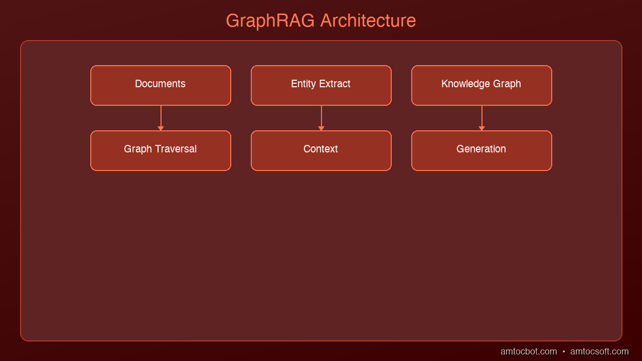
Architecture Diagram

GraphRAG, pioneered by Microsoft Research in 2024, adds a knowledge graph layer on top of traditional retrieval. The process has two phases:

Phase 1: Indexing (Building the Graph)

Documents → Chunk → Extract Entities & Relationships → Build Knowledge Graph → Detect Communities → Generate Community Summaries

1. Entity Extraction: An LLM reads each chunk and extracts named entities (people, organizations, concepts, technologies) and the relationships between them.

2. Knowledge Graph Construction: Entities become nodes, relationships become edges. "Claude" → DEVELOPED_BY → "Anthropic" becomes a directed edge in the graph.

3. Community Detection: Algorithms like Leiden clustering group tightly connected entities into communities. A cluster of related security concepts forms one community; a cluster of AI framework entities forms another.

4. Community Summaries: An LLM generates natural language summaries for each community, capturing the high-level themes and relationships within that cluster.

Phase 2: Querying

When a user asks a question, GraphRAG can use two strategies:

Local Search — Similar to traditional RAG but graph-enhanced:

  • Find relevant entities in the graph
  • Traverse their relationships to gather connected context
  • Retrieve the original text chunks associated with those entities
  • Feed everything to the LLM

Global Search — The game-changer:

  • Use community summaries to answer high-level questions
  • The LLM reads across community summaries to synthesize a global answer
  • No single chunk needs to contain the full answer

The Architecture Difference

Traditional RAG:
  Query → Embed → Vector Search → Top-K Chunks → LLM → Answer

GraphRAG (Local):
  Query → Entity Recognition → Graph Traversal → Related Chunks + Relationships → LLM → Answer

GraphRAG (Global):
  Query → Community Map → Relevant Summaries → LLM Synthesis → Answer

When to Use Which

| Scenario | Traditional RAG | GraphRAG |

|----------|----------------|----------|

| "What is our refund policy?" | Best choice | Overkill |

| "Summarize themes across 500 support tickets" | Poor — retrieves fragments | Excellent — uses community summaries |

| "How are Team A's projects connected to Team B's roadmap?" | Cannot connect across docs | Built for this — graph traversal |

| "Find the definition of Term X" | Best choice | Unnecessary |

| "What are the indirect dependencies of Service Y?" | Misses transitive relationships | Follows the dependency chain |

| "Which topics come up together in customer complaints?" | Retrieves individual complaints | Identifies co-occurring themes |

Rule of thumb: If the answer lives in a single passage, use traditional RAG. If the answer requires connecting information across multiple documents, use GraphRAG.

Building a Minimal GraphRAG Pipeline

Here's a simplified implementation using NetworkX and Claude:

import networkx as nx
import anthropic
from typing import List, Dict, Tuple

client = anthropic.Anthropic()

def extract_entities_and_relations(chunk: str) -> List[Dict]:
    """Use an LLM to extract entities and relationships from a text chunk."""
    response = client.messages.create(
        model="claude-sonnet-4-6-20250514",
        max_tokens=1024,
        messages=[{
            "role": "user",
            "content": f"""Extract entities and relationships from this text.
Return JSON array of objects with: source, relation, target

Text: {chunk}

Return only valid JSON."""
        }]
    )
    import json
    return json.loads(response.content[0].text)

def build_knowledge_graph(chunks: List[str]) -> nx.DiGraph:
    """Build a knowledge graph from document chunks."""
    G = nx.DiGraph()

    for i, chunk in enumerate(chunks):
        triples = extract_entities_and_relations(chunk)
        for triple in triples:
            G.add_edge(
                triple["source"],
                triple["target"],
                relation=triple["relation"],
                source_chunk=i
            )
    return G

def local_search(G: nx.DiGraph, query_entities: List[str],
                 chunks: List[str], hops: int = 2) -> str:
    """Graph-enhanced local search: find entities, traverse, gather context."""
    relevant_chunks = set()

    for entity in query_entities:
        if entity in G:
            # Get neighbors within N hops
            for neighbor in nx.single_source_shortest_path(G, entity, cutoff=hops):
                # Collect chunks associated with edges to this neighbor
                for _, _, data in G.edges(neighbor, data=True):
                    relevant_chunks.add(data.get("source_chunk"))

    # Build context from related chunks
    context = "\n---\n".join(chunks[i] for i in relevant_chunks if i < len(chunks))
    return context

# Usage
chunks = [...]  # Your document chunks
G = build_knowledge_graph(chunks)

# Query with graph-enhanced retrieval
context = local_search(G, ["Claude", "MCP"], chunks, hops=2)
response = client.messages.create(
    model="claude-sonnet-4-6-20250514",
    max_tokens=2048,
    messages=[{
        "role": "user",
        "content": f"Context:\n{context}\n\nQuestion: How does Claude use MCP?"
    }]
)

The Cost-Quality Tradeoff

GraphRAG is significantly more expensive than traditional RAG:

| Dimension | Traditional RAG | GraphRAG |

|-----------|----------------|----------|

| Indexing cost | Embedding API calls only | LLM calls for entity extraction + embeddings |

| Indexing time | Minutes for 10K docs | Hours for 10K docs (LLM-intensive) |

| Storage | Vector DB | Vector DB + Graph DB |

| Query latency | 100-500ms | 500ms-5s (graph traversal + LLM) |

| Query cost | 1 LLM call | 1-3 LLM calls (entity extraction + synthesis) |

| Global queries | Poor quality | High quality |

| Local queries | Good quality | Slightly better quality |

Microsoft's research showed GraphRAG outperformed traditional RAG by 30-70% on global sensemaking queries, but the indexing cost was 10-100x higher.

Real-World Applications

Corporate Knowledge Management: "What are the recurring themes across our last 12 months of board meeting minutes?" GraphRAG builds entity graphs across all meetings, identifies theme communities, and synthesizes a coherent answer no single document contains.

Biomedical Research: "What proteins interact with Drug X, and which of those are also targets of Drug Y?" The knowledge graph captures protein-drug-gene relationships across thousands of papers.

Supply Chain Analysis: "If Supplier A goes offline, what's the cascading impact on our product lines?" GraphRAG traces the dependency chain through the supply graph.

Legal Discovery: "Find all communications between these 5 people that reference Project Z." Graph search connects person nodes through communication edges filtered by topic.

Current Tools and Frameworks

| Tool | Type | Best For |

|------|------|----------|

| Microsoft GraphRAG | Full framework (Python) | Production-ready, well-documented |

| LlamaIndex | Property graph support | Integration with existing LlamaIndex pipelines |

| Neo4j + LangChain | Graph DB + framework | When you already use Neo4j |

| LightRAG | Lightweight alternative | Faster indexing, simpler setup |

| nano-graphrag | Minimal implementation | Learning and prototyping |

Start here: If you're exploring, try nano-graphrag to understand the concepts. For production, Microsoft's GraphRAG or LlamaIndex's property graph module.

The Hybrid Approach

The smartest teams don't choose one or the other. They use a routing layer that analyzes the query and decides which retrieval strategy to use:

def route_query(query: str) -> str:
    """Determine whether to use vector RAG or GraphRAG."""
    response = client.messages.create(
        model="claude-haiku-3-20250514",
        max_tokens=50,
        messages=[{
            "role": "user",
            "content": f"""Classify this query:
- "local" if it asks about a specific fact, definition, or passage
- "global" if it asks about themes, patterns, relationships, or summaries across multiple sources

Query: {query}
Classification:"""
        }]
    )
    return response.content[0].text.strip().lower()

# Route to appropriate strategy
if route_query(user_question) == "global":
    answer = graphrag_global_search(user_question)
else:
    answer = traditional_vector_search(user_question)

What's Next

GraphRAG is still evolving rapidly. The next frontier is dynamic graphs — knowledge graphs that update incrementally as new documents arrive, rather than requiring full reindexing. Combined with agentic RAG patterns (where an AI agent decides what to retrieve, from where, and when), we're moving toward retrieval systems that truly understand the structure of knowledge, not just the surface meaning of text.

If you're already running traditional RAG in production, the question isn't whether to switch — it's whether your users are asking questions that require connecting dots across documents. If they are, GraphRAG is worth the investment.

Sources & References:

1. Microsoft Research — "GraphRAG: Unlocking LLM Discovery on Narrative Private Data" (2024) — https://arxiv.org/abs/2404.16130

2. Microsoft — "GraphRAG GitHub Repository" — https://github.com/microsoft/graphrag

3. Lewis et al. — "Retrieval-Augmented Generation for Knowledge-Intensive NLP Tasks" (2020) — https://arxiv.org/abs/2005.11401

*Part of the RAG & Retrieval Systems series on [AmtocSoft](https://amtocsoft.blogspot.com). Follow us on [LinkedIn](https://www.linkedin.com/in/toc-am-b301373b4/) and [X](https://x.com/AmToc96282) for daily AI engineering insights.*


Enjoyed this post? Follow AmtocSoft for AI tutorials from beginner to professional.

Buy Me a Coffee | 🔔 YouTube | 💼 LinkedIn | 🐦 X/Twitter

Tuesday, March 31, 2026

How Transformers Work: The Architecture Behind Every Modern LLM

Level: Advanced | Topic: AI / ML Architecture | Read Time: 8 min

If you have used ChatGPT, Claude, Gemini, or any modern language model, you have interacted with a Transformer. Introduced in the 2017 paper "Attention Is All You Need" by Vaswani et al., the Transformer architecture replaced recurrent neural networks as the dominant approach for sequence modeling. Today, it powers everything from language models to image generators to protein folding predictions.

This article breaks down the core components of the Transformer architecture for developers who already understand basic neural network concepts and want to go deeper.

The Problem Transformers Solve

Before Transformers, sequence models like LSTMs and GRUs processed tokens one at a time, left to right. This sequential processing created two problems: it was slow (no parallelization) and it struggled with long-range dependencies. Transformers solve both by processing all positions simultaneously through self-attention, allowing every token to directly attend to every other token regardless of distance.

1. Input Embeddings and Positional Encoding

The Transformer converts each input token into a dense vector. Since the architecture processes all tokens in parallel, it has no inherent sense of order. Positional encodings are added to inject information about where each token sits in the sequence. Modern models use learned positional embeddings or rotary position embeddings (RoPE) for handling variable sequence lengths.

2. Self-Attention — The Core Innovation

For each token, the model computes three vectors: Query (Q), Key (K), and Value (V). The attention score between two tokens is the dot product of one token's Query with another's Key, scaled and passed through softmax. The output is a weighted sum of Value vectors. This allows the model to dynamically focus on the most relevant parts of the input for each position.

3. Multi-Head Attention

Rather than a single attention function, Transformers use multiple "heads" in parallel. Each head learns different patterns: syntactic relationships, semantic similarity, or positional proximity. The outputs are concatenated and projected. GPT-3, for example, uses 96 attention heads per layer.

4. Feed-Forward Network

After attention, each position passes through a two-layer MLP with a nonlinear activation. The FFN is where much of the model's factual "knowledge" is stored. Research suggests individual neurons activate for specific concepts learned during training.

5. Layer Norm and Residual Connections

Each sub-layer is wrapped with residual connections and layer normalization. Residual connections allow gradients to flow through very deep networks. Modern models use "pre-norm" design for more stable training at scale.

6. Decoder Stack and Output

In decoder-only models (GPT, LLaMA, Claude), causal attention ensures each token only attends to previous tokens, enabling autoregressive generation. The final layer projects to a vocabulary-sized probability distribution over the next token.

Why It Matters for Practitioners

Context window limitations stem from self-attention's O(n^2) cost. Techniques like Flash Attention and sparse attention are engineering solutions to this. Prompt engineering works because of how attention patterns form — the model learns which tokens are most relevant to generating each output token.

Key Takeaways

The Transformer architecture consists of embedding layers with positional encoding, multi-head self-attention for capturing relationships between all tokens, feed-forward networks for storing learned knowledge, and residual connections with layer normalization for stable training. Every major LLM today is built on this foundation.

If you found this useful, follow AmtocSoft for more content spanning AI, security, performance, and software engineering — from beginner to professional level.

Published by AmtocSoft | amtocsoft.blogspot.com

Context Packets for Production Agents: Keep the Model Small, Auditable, and Fast

Context Packets for Production Agents: Keep the Model Small, Auditable, and Fast Introduction: The Night the Prompt Became the Incide...