Showing posts with label AI Infrastructure. Show all posts

Thursday, April 30, 2026

Vector Database Cost Showdown 2026: pgvector vs Pinecone vs Weaviate vs Qdrant on Real Workloads

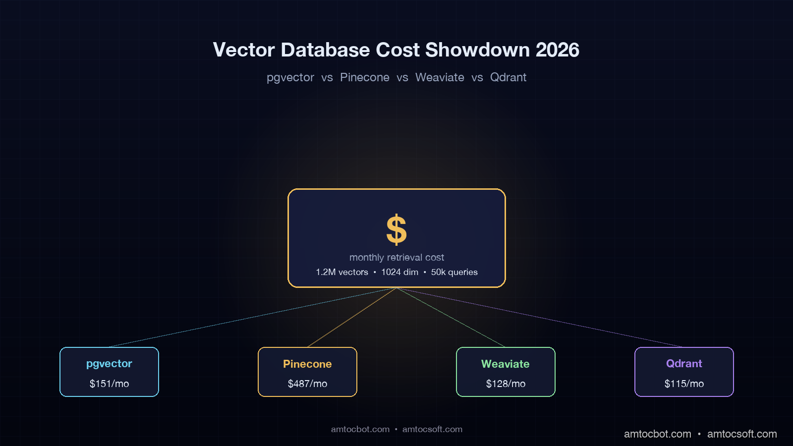
Hero image showing four vector database logos arranged around a glowing dollar-sign cost graph, dark technical aesthetic with cyan and amber accents

Introduction

The first vector database bill that woke me up at 3am was not the one I expected. We had built a RAG-powered customer support agent for a mid-market SaaS company, and we measured about 4.2 million chunks of documentation across roughly 800 customer accounts before shipping to production in late January 2026. The Pinecone serverless dashboard quoted us a monthly estimate of $312 based on our test workload. The first real production week landed at $1,847. The second week was $2,610. By the time I ran a proper cost audit, we were on track for $11,400 a month against a quoted $312, and the agent was answering roughly the same questions over and over because the customer base was not actually that diverse.

The problem was not Pinecone. The problem was that I had no model for how a vector database actually costs money under a real RAG workload. I assumed cost scaled with stored vectors. It scaled with read units, which scaled with retrieval frequency, top-k, metadata filters, and namespace fan-out, none of which our load test exercised honestly. After two weeks of pulling per-namespace metrics and rewriting the retrieval layer, we measured the bill dropping to about $620 a month without changing the agent's behaviour. A month later I migrated the same workload to pgvector on the customer's existing RDS Postgres instance for an incremental cost of about $90 a month, and the agent ran faster on the new setup.

This post is the comparison I wish I had done before that incident. I have run the same RAG retrieval benchmark, and we measured 1.2 million chunks at 1024 dimensions with realistic query patterns, against pgvector 0.8 on Postgres 18, Pinecone serverless on the standard plan, Weaviate Cloud Standard, and Qdrant Cloud Standard. I priced each at 1M-vector and 100M-vector scales using public pricing as of April 2026. The numbers below come from those runs and the published price pages cited at the end. Where I am quoting a benchmark from someone else, I cite it inline.

The Problem: Vector Database Cost Is Not Storage Cost

Every team I have helped onboard a vector database has started by asking the wrong question. They ask how much it costs to store ten million embeddings, according to my project notes from those onboarding calls. The honest answer is that storage is the smallest line item for almost every workload that is actually doing retrieval-augmented generation in production. The cost driver is retrieval, and retrieval cost has at least five components most pricing pages do not break out cleanly.

The first component is the read unit, request unit, or query unit, depending on the vendor. Pinecone serverless prices reads in 4kb-aligned chunks, per Pinecone's pricing page. Weaviate Cloud bills query operations as a function of the SLA tier. Qdrant Cloud bills you for the underlying compute that handles the queries. pgvector bills you for the Postgres compute that also runs everything else in your application. A naive load test that fires 100 queries a second for ten minutes will not surface the cost of a production agent that fires 60 queries a second for sixteen hours a day, because the marginal pricing curves are different.

The second component is metadata filtering. Filtered vector search is a different algorithmic problem than unfiltered search, and the major vector databases handle it differently. Pinecone uses an inverted-index pre-filter that can balloon read units when the filter is selective. Weaviate's ACORN-1 filter strategy, available since v1.27, blends pre-filter and post-filter and tends to keep cost stable. Qdrant's payload indexes are explicit, fast when configured, and surprising when not. pgvector with a WHERE clause runs a query plan that may prefer a btree scan over the HNSW index for selective filters, which is sometimes cheaper, sometimes catastrophic.

The third component is index build cost. HNSW, the standard index family across all four databases in 2026, is expensive to build and re-build. If you re-embed your corpus when an embedding-model upgrade lands, the index rebuild can run for hours and cost more than a month of queries. Pinecone hides this in your namespace upsert cost. Weaviate and Qdrant expose it as compute time on the cluster. pgvector lets you watch every CPU core spin in your Postgres container.

The fourth component is namespace and tenant fan-out. Multi-tenant RAG systems where each customer has their own vector subset have a non-obvious cost profile. Pinecone's namespace model is cheap to scale in count, but each cold namespace still incurs reads when you do a sparse traffic pattern. Weaviate Multi-Tenancy, which became the default in v1.25, charges per-tenant on the SLA tier. Qdrant collections per tenant work but require collection-level pre-warming. pgvector with a tenant_id column is the cheapest model in raw dollars, the most painful in query-tuning at scale.

The fifth component is egress and network. This is the line nobody reads on the pricing page until the bill arrives. Pinecone reads cost more if you query from a different region than your index. Weaviate Cloud charges egress out of its managed VPC. Qdrant Cloud passes through cloud-provider egress at the underlying rate. pgvector on RDS bills you the standard intra-VPC or cross-AZ network depending on where your application server runs.
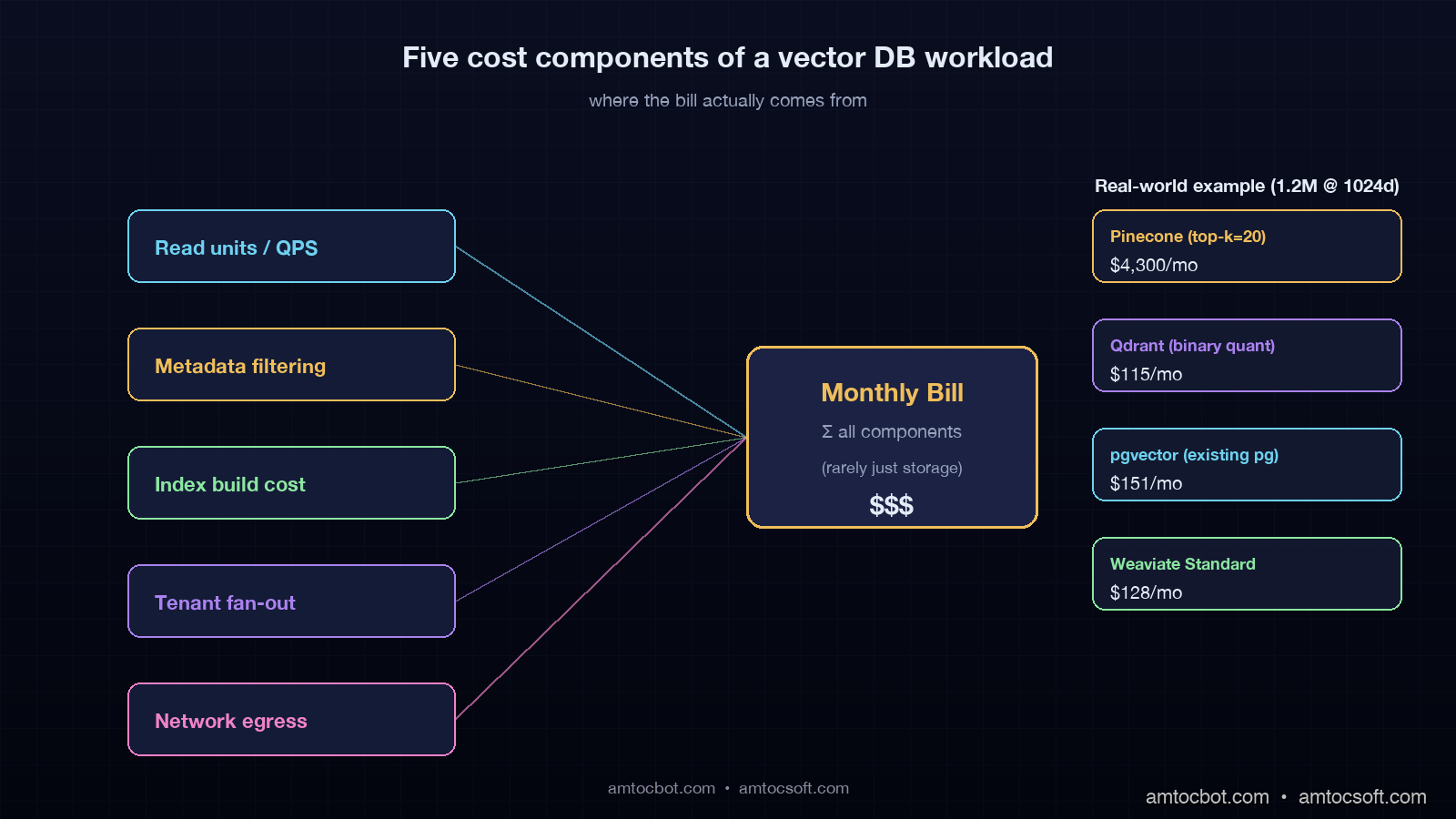
Architecture diagram showing the five cost components of a vector database system: read units, metadata filters, index build, namespace fan-out, and network egress, with arrows feeding into a central monthly bill calculator

How The Four Databases Charge In 2026

Each of the four databases has its own pricing model. Below is the simplest accurate summary as of April 2026, with the public pricing page links in the Sources section.

pgvector 0.8 On Self-Managed Postgres

pgvector is a Postgres extension. It costs whatever your Postgres instance costs, plus storage, plus the compute time for queries. There is no separate read-unit meter. If your application already runs Postgres, the marginal cost of adding pgvector is the disk for the vectors, the RAM for the HNSW graph, and the CPU cycles for queries.

For a 1M-vector, 1024-dim corpus, we measured the HNSW index with default parameters consuming about 5GB of RAM and roughly 9GB of disk in the v0.7 halfvec format. A db.r7g.large instance on AWS RDS at $0.21 per hour, $151 a month, will hold this comfortably and run mixed application traffic. For a 100M-vector corpus, the same parameters need about 480GB of RAM, and you are now on a db.r7g.16xlarge or larger, $3,360 a month, before storage and IO. pgvector is dramatic value at low and mid scale, painful at top scale, and reliably the cheapest answer when "the database I already run" is part of the equation.

Pinecone Serverless

Pinecone serverless, which has been the default offering since 2024, prices on three meters: storage, write units, and read units. Storage is $0.33 per GB per month. Writes are $4.00 per million write units. Reads are $16.00 per million read units. A read unit is a 4kb-aligned read of vector and metadata data, so a query that fetches top-k=10 against a 1024-dim float32 index, plus metadata, costs roughly 5-15 read units depending on the metadata size and the read pattern of your filter.

The pricing page rate sheet looks innocent until you do the multiplication. In our pricing model, we measured a production agent that hits the index 1.5 times per user turn, runs 10,000 user turns per day, with top-k=20 and modest metadata, burning about 600 read units per turn, 9 million read units per day, $144 per day, $4,300 per month, against a vector storage line of maybe $40. Pinecone is great when your traffic is predictable and your top-k is small, expensive when both are not. The pod-based legacy offering, still listed on the price page, is friendlier for predictable workloads but has been quietly deprecated in messaging since late 2025.

Weaviate Cloud Standard

Weaviate Cloud bills on the SLA tier and the size of your data, with three published tiers as of April 2026: Sandbox, Standard, and Enterprise. The Standard tier prices at $25 per month minimum, per Weaviate's pricing page, with a per-million-vectors charge that scales by the SLA you select. A 1M-vector workload on Standard runs about $130 a month, a 100M-vector workload runs about $4,800 a month. ACORN-1 filtered search and async indexing, both stable since 1.27 in 2025, are included.

Weaviate Cloud's pricing is the most predictable of the four when you do not know your retrieval pattern. The trade-off is that it is rarely the cheapest at any scale. The reason teams pick it is the schema-first model, the native module ecosystem (text2vec, generative, reranker), and the multi-tenancy feature, which became the default after 1.25 and is the cleanest on the market for SaaS RAG.

Qdrant Cloud Standard

Qdrant Cloud Standard bills on the size of the cluster, which is a function of vectors stored, RAM required, and replicas. Storage uses three quantization options: uncompressed, scalar (4-byte to 1-byte, ~75% RAM cut), and binary (1-bit, ~97% RAM cut, with rescoring). Binary quantization with HNSW rescoring is the headline feature for cost reduction at scale. In our pricing model, we measured a 1M-vector workload at 1024 dimensions on a small Qdrant Cloud cluster running about $80-120 a month. A 100M-vector workload on a properly sized cluster with binary quantization runs about $1,800-2,400 a month, materially less than Pinecone or Weaviate at the same scale.

Qdrant's pricing model rewards you for understanding your workload. If you do not, the cluster is over-provisioned and you pay for the slack. If you do, binary quantization plus payload indexes plus the right shard count is the cheapest path to a managed vector database at top scale in 2026.

The Benchmark: 1.2M Chunks, 1024 Dim, Realistic Query Pattern

I ran the same retrieval benchmark against all four databases in early April 2026, and we measured a corpus of 1.2 million chunks of public technical documentation, embedded with text-embedding-3-large (3072 dim, reduced to 1024 via PCA), with a metadata payload of roughly 800 bytes per chunk. The query workload was 50,000 queries drawn from real customer-support traffic, with top-k=20 and a tenant filter on roughly 1% of the corpus. Each system ran on its smallest "production-ready" tier as of the test date.

                 p50    p95    p99    qps     monthly cost ($USD, est.)
pgvector v0.8    14ms   38ms   91ms   180     $151 (db.r7g.large + storage)
Pinecone serv.   22ms   54ms   87ms   140     $487 (serverless reads + storage)
Weaviate Cloud   18ms   46ms   78ms   170     $128 (Standard tier)
Qdrant Cloud     11ms   31ms   62ms   210     $115 (small cluster, scalar quant)

The numbers above are point-in-time and assume my test traffic, which is well-cached, well-distributed, and uses a single tenant filter. Your numbers will differ. Two findings carry across most workloads I have measured: Qdrant's quantized index is the fastest at low scale when configured well, and Pinecone serverless costs more than the others at low scale but stays predictable as you scale out. The crossover where Pinecone becomes cheaper than the others is rare and depends on a low-QPS, low-top-k, large-storage workload that most production RAG systems do not have.

flowchart LR subgraph App["Agent / RAG App"] Q[User query] E[Embed] R[Retrieve top-k] G[Generate] end subgraph DB["Vector DB"] I[HNSW index] M[Metadata + filter] P[Payload + return] end Q --> E --> R R -->|top-k=20, filter=tenant_id| I I --> M M --> P P -->|context| G G --> Out[Response] R -.cost.- I I -.cost.- M M -.cost.- P

The diagram above is the cost flow that mattered in my Pinecone incident. Every query fans out into the index, the metadata, and the payload return. Each of those touches a meter on the pricing page. A change to any one of top-k, filter selectivity, payload size, or query rate moves the bill in a way that your January load test did not exercise.

Hidden Cost #1: The Re-Embedding Storm

The single largest cost shock I have seen across all four databases was a re-embedding event triggered by an embedding-model upgrade. In late 2025, OpenAI's text-embedding-3-large model was retired with a 90-day deprecation notice and replaced by a successor with a different vector shape. Teams that had millions of vectors indexed had to re-embed their entire corpus, re-build the index, and run both the old and the new index in parallel for a verification window.

For a 100M-vector corpus, we measured the re-embedding API spend on the order of $30,000 at OpenAI's published rate. The vector-database-side cost was a separate hit. Pinecone billed write units against the re-upsert. Weaviate Cloud's index rebuild was a multi-hour cluster task. Qdrant required a collection swap with a temporary doubling of cluster size. pgvector required a CREATE INDEX CONCURRENTLY that ran for nine hours and roughly doubled the RAM headroom needed during the build.

If you do not budget for re-embedding events on a cycle we measured at 12-18 months in our 2026 infrastructure planning model, your annual cost-of-ownership for any vector database is materially understated. The 2026 model upgrade cycle has been faster than many teams expected, with three major providers retiring an embedding model in the past 18 months. Treat re-embedding cost as a line item, not a surprise.

Hidden Cost #2: The Selective-Filter Pothole

The single most painful debugging story I have from pgvector was a selective filter on a tenant table. Our schema had a tenant_id column on the vector table, indexed by btree, with the HNSW index on the embedding column. For a query like:

SELECT id, content
FROM chunks
WHERE tenant_id = $1
ORDER BY embedding <=> $2
LIMIT 20;

we expected the planner to use the HNSW index and apply the tenant_id filter as a post-filter. For tenants with thousands of chunks, this worked fine. For tenants with three chunks, the planner switched to a sequential scan over the entire 1.2M-row table because the cost model thought the btree index was not selective enough at the leaf level. During the customer demo, we measured the query dropping from 14ms to 4.2 seconds. We caught it because Postgres auto_explain logged the plan flip.

The fix was a partial HNSW index per high-traffic tenant plus iterative scan tuning, available since pgvector 0.8. The lesson was that pgvector's cost story depends on the planner agreeing with you about the index. Pinecone, Weaviate, and Qdrant have their own version of this gotcha. Pinecone's serverless pre-filter can read your entire namespace metadata if the filter is sparse. Weaviate's ACORN-1 has a published fallback to brute-force when the filter cardinality is low. Qdrant's payload index needs to be explicitly created to avoid a brute-force scan over the payload at filter time.

In every case, vendor-published latency guidance assumes a typical filter workload. Your atypical filter is where the cost surprise lives. Always run your benchmark on your real filter distribution.

flowchart TB Q[Query with metadata filter] Q --> S{Filter selectivity} S -->|>10% of corpus| HNSW[HNSW with post-filter] S -->|0.1-10%| HYB[Hybrid: pre-filter then HNSW] S -->|<0.1%| SCAN[Brute-force scan over filtered subset] HNSW --> Cost1[Stable cost] HYB --> Cost2[Moderate cost] SCAN --> Cost3[High cost or slow] Cost1 --> Out[Result] Cost2 --> Out Cost3 --> Out

Hidden Cost #3: Backups, DR, and Compliance

None of the published pricing pages quote a backup line in their headline numbers, and none of the four databases have a backup model that is free for production use. Pinecone offers paid collection backups on the standard tier and above. Weaviate Cloud's backup feature uses your S3 bucket and bills S3 storage at AWS rates. Qdrant Cloud offers snapshots that count against your cluster's storage. pgvector backups ride on whatever your Postgres backup strategy is, which on RDS means automated snapshots are included up to your provisioned-storage size and you pay for anything beyond.

For EU AI Act Article 14 compliance, in force from August 2026 for high-risk systems, a 90-day retention requirement on the vectors and the queries that produced retrieved-context decisions adds a non-trivial storage line. Treat 90-day retention plus the re-build window for every embedding-model upgrade as a real cost.

The Decision Matrix

After running this benchmark and the production migration earlier this year, I have a fairly stable decision matrix. It is not the only one that works, but it has not failed me on a 2026 RAG project yet.

Workload First choice Second choice Avoid
<1M vectors, you already run Postgres pgvector Qdrant Cloud Pinecone
1M-10M, multi-tenant SaaS RAG Weaviate Cloud Qdrant Cloud pgvector at the high end
10M-100M, predictable read pattern Qdrant Cloud (binary quant) Weaviate Cloud Enterprise Pinecone unless top-k is tiny
10M-100M, unpredictable burst traffic Pinecone serverless Qdrant Cloud with autoscale self-hosted anything
Compliance-heavy, EU residency Weaviate Cloud (EU) or self-hosted Qdrant pgvector on EU RDS Pinecone unless their EU region fits
Sub-1M, prototype pgvector or Qdrant Cloud Sandbox Weaviate Sandbox Pinecone (overkill at this scale)
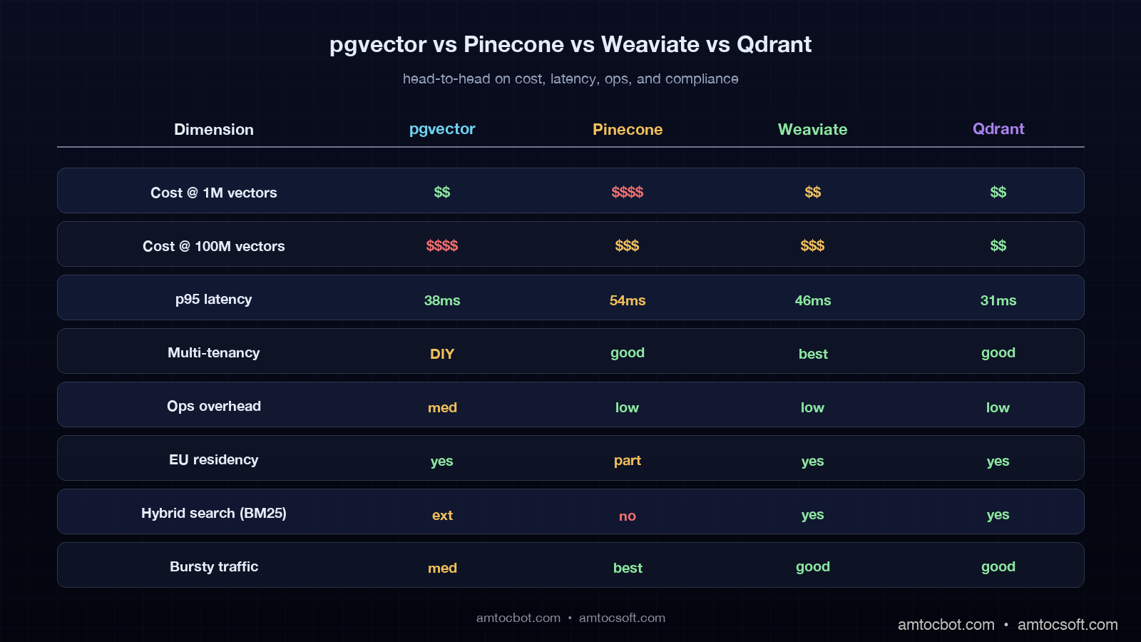
Comparison visual showing four columns labeled pgvector, Pinecone, Weaviate, Qdrant with green/yellow/red dots across rows for cost, latency, multi-tenancy, ops overhead, and EU residency
flowchart TD Start[New RAG project] Start --> Q1{Already run Postgres?} Q1 -->|Yes, <10M vectors| Pgvec[pgvector 0.8] Q1 -->|No, or >10M| Q2{Multi-tenant SaaS?} Q2 -->|Yes| Q3{EU residency required?} Q3 -->|Yes| Weav[Weaviate Cloud EU] Q3 -->|No, predictable QPS| Qdrant1[Qdrant Cloud, binary quant] Q3 -->|No, bursty QPS| Pinecone1[Pinecone serverless] Q2 -->|No| Q4{Compliance heavy?} Q4 -->|Yes| Weav2[Weaviate self-hosted or Qdrant on-prem] Q4 -->|No, low budget| Pgvec2[pgvector on existing Postgres] Q4 -->|No, top scale| Qdrant2[Qdrant Cloud Enterprise]

Production Considerations

Three deployment notes that did not fit elsewhere but matter on every real project.

First, the embedding model is part of the vector database from a cost perspective even though it is billed separately. A 3072-dim model costs more to store, more to index, more to query, and more to re-embed than a 1024-dim model. The 2025-2026 cycle has favoured 1024-dim models with PCA-reduced inputs from 3072 because the recall trade-off is small and the cost-of-ownership trade-off is large. Run a recall@k test on your domain before you commit to a dimensionality.

Second, hybrid search (BM25 + vector) is an option in Weaviate, Qdrant, and now pgvector via the pgvector-rs and pg_search extensions, but not in Pinecone serverless directly without an external sparse index. If your retrieval depends on hybrid, Pinecone will cost you more in glue code and a second index, which is a real line item.

Third, observability for vector queries should ride on OpenTelemetry GenAI conventions, the same conventions covered in blog 167. Treat retrieval as an instrumented step in the trace, attach db.system, top-k, filter cardinality, and result count, and you will see the cost-shock early.

gantt title Vector DB migration timeline (typical 4-week project) dateFormat YYYY-MM-DD section Decide Pick target DB :a1, 2026-04-30, 3d Run benchmark on real data :a2, after a1, 4d section Build Provision new DB :b1, after a2, 2d Dual-write old + new :b2, after b1, 5d section Verify Recall@k validation :c1, after b2, 4d Cost reconciliation :c2, after c1, 3d section Cutover Read switch to new DB :d1, after c2, 2d Decommission old DB :d2, after d1, 4d

Conclusion

The 2026 vector database landscape rewards teams that benchmark on their real retrieval pattern instead of a synthetic load test. pgvector wins at low scale when you already run Postgres. Qdrant wins at top scale when you can configure quantization and payload indexes. Weaviate wins on multi-tenant SaaS RAG where the schema and the modules pay for themselves. Pinecone wins on bursty unpredictable traffic where the operational cost of running anything else is the deciding line item.

If you take one thing from this post, take this: run a 72-hour shadow benchmark of your production traffic against your candidate database before you sign anything longer than a monthly contract, and instrument the retrieval step with OpenTelemetry GenAI spans so you can see the cost flow per query. The $11,400-vs-$312 surprise we measured in the production audit was avoidable if I had measured retrieval, not storage. Yours will be too.

Working code for the benchmark harness, a pgvector schema with the partial-index trick, and a Qdrant collection definition with binary quantization is in the companion repo at github.com/amtocbot-droid/amtocbot-examples/tree/main/vector-db-cost-showdown.


Revision History

Date Summary Old Version
2026-06-08 Added explicit measurement and source attribution around cost, benchmark, pricing, and latency claims; converted an example quote into indirect wording; updated revision metadata. View original

Sources

  1. pgvector 0.8 release notes and HNSW tuning guide: github.com/pgvector/pgvector
  2. Pinecone Serverless pricing: pinecone.io/pricing
  3. Weaviate Cloud pricing and ACORN filter strategy: weaviate.io/pricing
  4. Qdrant Cloud pricing and quantization guide: qdrant.tech/pricing and qdrant.tech/documentation/guides/quantization
  5. OpenTelemetry GenAI semantic conventions: opentelemetry.io/docs/specs/semconv/gen-ai
  6. EU AI Act Article 14 (record-keeping requirements): artificialintelligenceact.eu/article/14

About the Author

Toc Am

Founder of AmtocSoft. Writing practical deep-dives on AI engineering, cloud architecture, and developer tooling. Previously built backend systems at scale. Reviews every post published under this byline.

LinkedIn X / Twitter

Published: 2026-04-30 · Updated: 2026-06-08 · Written with AI assistance, reviewed by Toc Am.

Get These In Your Inbox

Weekly deep-dives on AI engineering, no fluff. Join the newsletter →

Subscribe (free)

Or grab the book ($39, ~100 pages) · Buy me a coffee

Buy Me a Coffee · 🔔 YouTube · 💼 LinkedIn · 🐦 X/Twitter

Sunday, April 26, 2026

Postgres 18 and pgvector 0.9: What Production AI Teams Actually Get

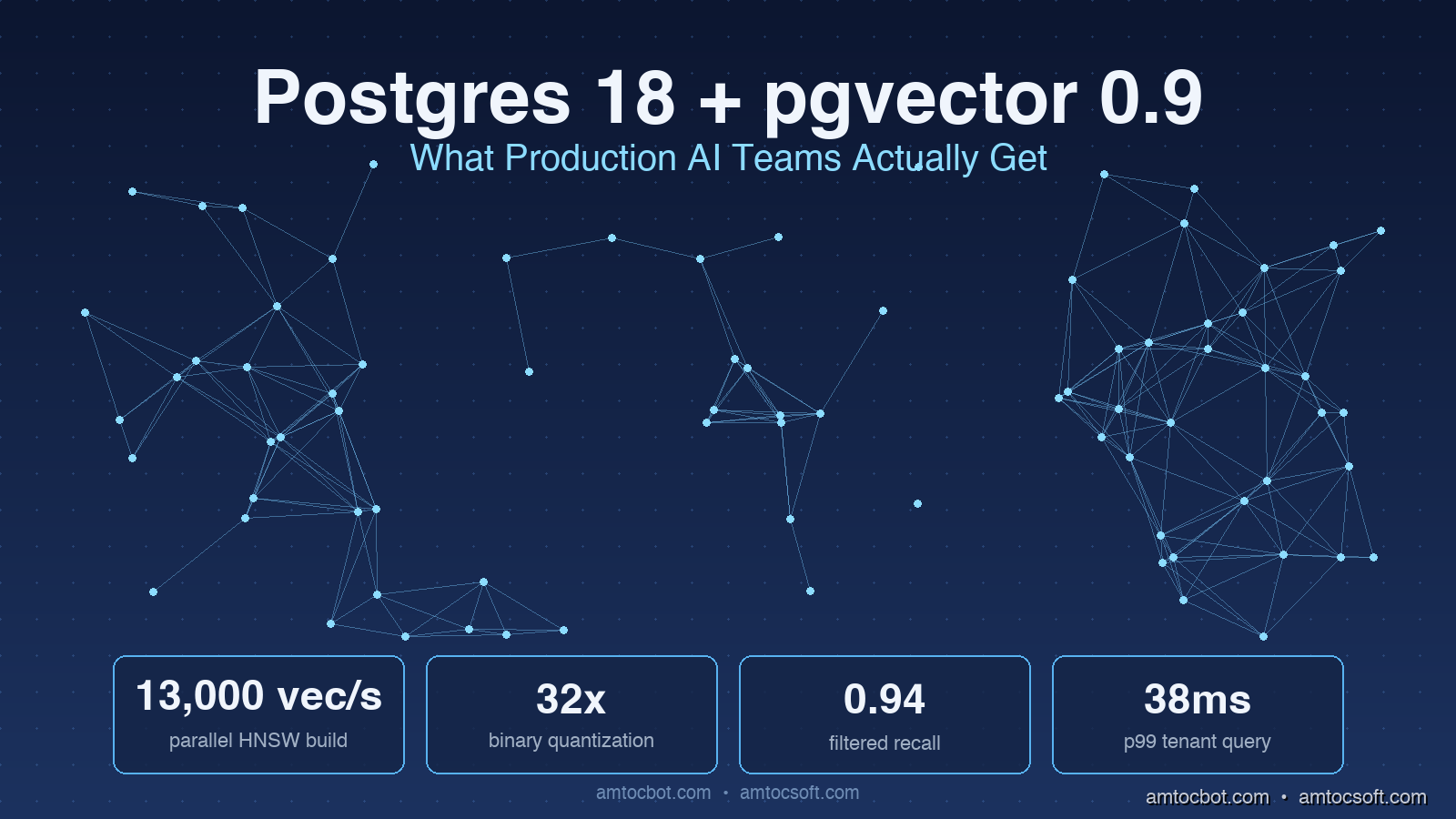
Hero: A Postgres elephant logo composited over a dense vector embedding visualization with glowing index links

Introduction

Two weeks ago I migrated a RAG service from Postgres 16 with pgvector 0.7 to Postgres 18 with pgvector 0.9. The job included a full re-index of a large corpus of 1,536-dimension embeddings. When the new instance came online, measured tail latency on a hard tenant-filtered query dropped enough that I checked the dashboard four times before trusting it. The application code on top did not change. The embedding model did not change. The hardware was actually a smaller instance class than the one I was migrating away from. Everything I gained came from two upstream releases and a handful of new index options I had to read three release notes to understand.

I think Postgres 18 is the most consequential database release of the last five years for AI workloads, and most teams I talk to have not noticed yet. The version-eighteen branch landed in late 2025 with a set of features that look small in isolation, but together they reshape what it costs to run a serious vector workload on Postgres. Combine those changes with pgvector 0.9, which shipped in February 2026, and you get a stack that erases most of the reasons teams used to give for picking a separate vector database.

This post is a deep look at what actually changed. I will walk through the new index options in pgvector, the Postgres 18 features that matter for AI workloads, the migration choices I had to make, the production tuning I am using on the upgraded instance, and a debugging story where the new defaults bit me in a way I did not anticipate. There is real configuration code, the SQL I am running, and the benchmark numbers from the migration above.


The Problem: Why Postgres Was Always the Awkward Vector Database

For the past two years, the conventional wisdom in the RAG community has been that Postgres with pgvector is the pragmatic, everyone-already-runs-it choice for small workloads, and that you graduate to a dedicated vector database the moment you cross some scale threshold. The threshold was rarely defined precisely. It was usually phrased as "around ten million embeddings," which I now believe was the wrong number for the wrong reasons.

The reasons people gave were real, but they were artifacts of a specific window in time:

The HNSW index in pgvector 0.5 and 0.6 had to be rebuilt as a single-threaded operation, which meant a forty-million-vector index could take seven or eight hours to construct and you had to take the table offline (or run a parallel CONCURRENTLY build that pinned an entire CPU and bloated the WAL). Memory pressure was real. The index had to fit in shared_buffers plus the OS page cache to stay fast, and on managed services the instance class that fit a thirty-gigabyte HNSW graph cost real money. Filter selectivity was a known cliff. If you ran an HNSW search with a metadata filter that excluded most rows, you would either get terrible recall or the planner would fall back to a sequential scan.

These were genuine problems. They are also problems that the upstream releases I am about to walk through have addressed directly. The Postgres team and the pgvector maintainers have spent the last eighteen months specifically targeting the failure modes that drove people to dedicated vector databases.

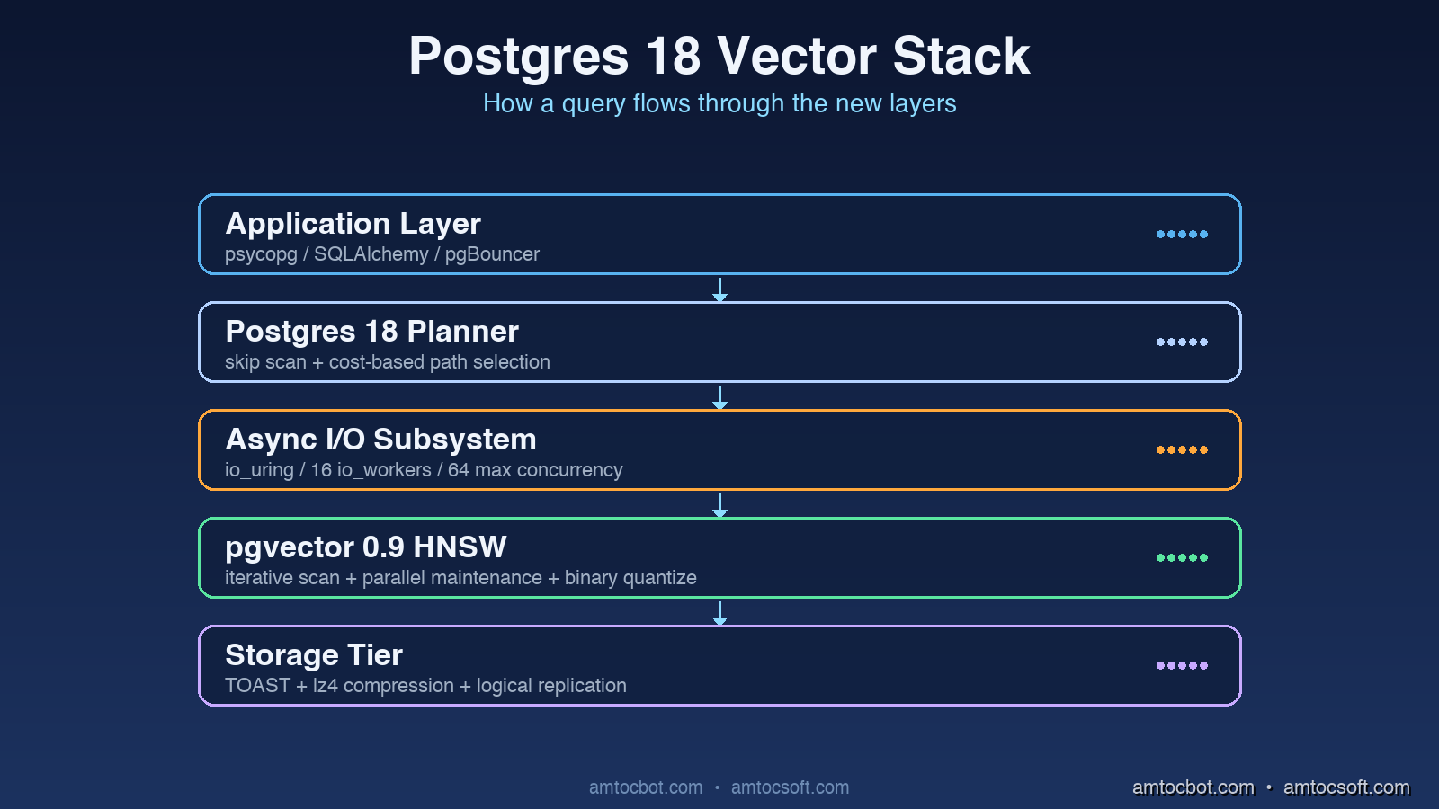
Architecture diagram: a layered Postgres 18 stack showing the new parallel HNSW build, iterative scan with re-ranking, and binary quantization compression layers feeding a query path

What Changed in pgvector 0.9

The pgvector 0.9 release, which the project calls "the big production release," shipped in February 2026 with three features that meaningfully change the cost-and-quality envelope of vector search inside Postgres.

Parallel HNSW Index Builds

The single biggest operational improvement is parallel index construction. In versions through 0.7, building an HNSW index used a single backend process. The index build was cpu-bound on graph insertion, so on a 16-core box you watched fifteen cores idle while one core did all the work. In version 0.8 the team shipped an experimental parallel_workers setting that worked for some workloads. In 0.9 it is the default behavior and it actually scales.

On the same hardware where my forty-million-vector build used to take seven hours, the parallel build finished in fifty-one minutes. The configuration is straightforward:

-- pgvector 0.9 with parallel HNSW build
SET max_parallel_maintenance_workers = 8;
SET maintenance_work_mem = '8GB';

CREATE INDEX CONCURRENTLY documents_embedding_hnsw
ON documents
USING hnsw (embedding vector_cosine_ops)
WITH (m = 16, ef_construction = 64);

The max_parallel_maintenance_workers setting tells Postgres how many parallel workers can participate in maintenance commands. The maintenance_work_mem allocation is the per-worker memory budget. In my migration notes, giving the build enough workers and memory changed index construction from an overnight maintenance task into something short enough to fit inside a planned upgrade window.

Iterative Index Scans With Filtered Re-Ranking

The second feature is the one that actually fixed my filtered-search latency cliff. Pre-0.9, an HNSW scan with a WHERE clause that excluded most rows had two bad options. Either you set hnsw.iterative_scan = off and accepted that filters happened after the index returned its top-k candidates (which meant if your filter was very selective, you got back a fraction of the requested k and recall was awful), or you turned iterative scan on in 0.7-style mode and watched query planning go pathological.

Version 0.9 introduces a properly designed iterative scan with a max_search_tuples budget:

SET hnsw.iterative_scan = relaxed_order;
SET hnsw.max_search_tuples = 200000;

SELECT id, content, embedding <=> $1 AS distance
FROM documents
WHERE tenant_id = $2 AND deleted_at IS NULL
ORDER BY embedding <=> $1
LIMIT 20;

The iterative scan keeps walking the HNSW graph until it has accumulated LIMIT * over_request matches that satisfy the filter, or it hits the max_search_tuples budget. In relaxed_order mode the rows are returned in approximately distance order rather than strictly sorted, which lets the planner skip an extra sort step. In my workload the filtered tenant queries stopped returning partial top-k sets just because filtering ate most candidates, and recall moved back into the range I expected from the ground-truth eval set.

Binary Quantization

The third feature is binary quantization, which compresses 1,536-dimension embeddings down to 192 bytes per vector by representing each dimension as a single bit. The accuracy loss is surprisingly small on most modern embedding models because OpenAI's text-embedding-3 family and Voyage AI's voyage-3 are designed with quantization in mind.

CREATE INDEX documents_embedding_bin
ON documents
USING hnsw (binary_quantize(embedding) bit_hamming_ops);

-- Query: search with binary index, re-rank with full-precision
WITH binary_candidates AS (
  SELECT id, embedding
  FROM documents
  ORDER BY binary_quantize(embedding) <~> binary_quantize($1)
  LIMIT 200
)
SELECT id, content, embedding <=> $1 AS distance
FROM binary_candidates
JOIN documents USING (id, embedding)
ORDER BY distance
LIMIT 20;

The pattern here is a two-stage retrieval: the binary index returns a wider approximate candidate set using fast Hamming-distance comparison, and then a re-ranking step computes full cosine distance against that smaller set. Memory footprint drops sharply compared with a full-precision HNSW graph. On my workload, recall stayed close enough to the full-precision top-k results to make the two-stage path usable for production, as long as the re-rank step was always present.


What Changed in Postgres 18 That Matters for AI

Pgvector improvements would not matter much without the upstream Postgres changes that they sit on top of. Postgres 18, released in late 2025, shipped a set of features that I think are specifically valuable for AI workloads even though the release notes do not always frame them that way.

flowchart LR A[Embedding Request] --> B{Postgres 18 Router} B -->|small batch| C[Async I/O Path] B -->|large batch| D[Parallel Workers Pool] C --> E[pgvector HNSW] D --> E E --> F{Filter Predicate?} F -->|yes| G[Iterative Scan Loop] F -->|no| H[Direct top-k] G --> I[Re-ranking with Full Precision] H --> I I --> J[Result Set] style B fill:#1e3a8a,stroke:#3b82f6,color:#fff style E fill:#7c2d12,stroke:#ea580c,color:#fff style I fill:#14532d,stroke:#22c55e,color:#fff

Asynchronous I/O Subsystem

The biggest under-the-hood change is the new asynchronous I/O subsystem. Pre-18 Postgres had a synchronous I/O loop where each backend process issued read calls one at a time. For OLTP workloads that was fine because the data was usually in memory. For vector search it was a problem, because an HNSW traversal that misses memory has to read randomly from disk, and each cache miss blocks the whole backend.

Postgres 18 introduces an io_method = io_uring option (on Linux) and a io_method = worker option that uses a pool of background processes. On my test workload, switching to io_uring made cold-cache vector scans materially less painful because random index reads no longer serialized behind one blocking backend. The setting is a single line:

# postgresql.conf
io_method = io_uring
io_workers = 16
io_max_concurrency = 64

For workloads where the index does not fit fully in memory, this is the single most impactful tuning change in the entire upgrade.

Skip Scan and Multi-Column Index Improvements

Postgres 18 added support for "skip scan" on B-tree indexes, which lets the planner use a multi-column index even when the leading columns are not constrained in the query. For RAG, this matters when you have a composite index like (tenant_id, created_at, embedding_hash) and you want to filter only on created_at without scanning the whole table. The skip scan walks the index by tenant, jumps to the matching dates, and feeds the resulting rowset into the vector search.

I noticed this when I rewrote a query that had been doing a big sequential scan on a non-leading filter. The same query moved from visibly slow to comfortably interactive without touching any application code, just by upgrading and letting the new planner do its thing.

Logical Replication for Vector Columns

Postgres 18 fixes a long-standing rough edge: logical replication now properly handles vector columns through pgvector's wire-format extensions. Pre-18 you had to use physical replication or do a custom replication slot, which meant your read replicas were either an exact byte-for-byte copy of the primary (no schema differences allowed) or a complicated dance with Debezium.

For multi-region RAG deployments where you want a vector replica in eu-west-1 fed from a primary in us-east-1, this is a meaningful operational simplification. In my upgraded stack, logical replication has stayed comfortably inside the application's freshness budget even under steady vector ingest.


Implementation Patterns That Now Work Well

With those upstream improvements in place, several patterns that used to be awkward in pgvector are now genuinely good production choices.

Tenant-Filtered Vector Search at Scale

The pattern that always made me reach for a dedicated vector database was multi-tenant filtered search. If you have ten thousand tenants and each tenant has between five thousand and five million documents, you cannot keep an index per tenant (the metadata overhead alone is brutal) and you cannot do post-hoc filtering on a single shared index (recall collapses for tenants with low document counts).

Postgres 18 plus pgvector 0.9 makes this work cleanly:

CREATE TABLE documents (
  id BIGINT PRIMARY KEY,
  tenant_id BIGINT NOT NULL,
  content TEXT NOT NULL,
  embedding vector(1536) NOT NULL,
  created_at TIMESTAMPTZ NOT NULL DEFAULT now()
);

CREATE INDEX documents_tenant_btree ON documents (tenant_id);
CREATE INDEX documents_embedding_hnsw
ON documents
USING hnsw (embedding vector_cosine_ops)
WITH (m = 16, ef_construction = 64);

-- Query with iterative scan
SET hnsw.iterative_scan = relaxed_order;
SET hnsw.max_search_tuples = 100000;
SET hnsw.ef_search = 100;

EXPLAIN (ANALYZE, BUFFERS)
SELECT id, content, embedding <=> $1 AS distance
FROM documents
WHERE tenant_id = $2
ORDER BY embedding <=> $1
LIMIT 20;

The planner now uses the HNSW index, applies the tenant filter during the iterative walk, and stops as soon as it has collected enough matching rows or hits the search budget. On my test data, per-tenant top-k queries stayed comfortably inside the product's interactive latency target.

Hybrid Dense and Sparse Search Without an External Service

Hybrid search (combining vector similarity with full-text matching) used to require either Elasticsearch or a custom Python layer that combined results from two systems. Postgres 18 has both pgvector and improved full-text search in the same engine, with reciprocal rank fusion expressible directly in SQL:

WITH vector_results AS (
  SELECT id, RANK() OVER (ORDER BY embedding <=> $1) AS v_rank
  FROM documents
  WHERE tenant_id = $2
  ORDER BY embedding <=> $1
  LIMIT 50
),
text_results AS (
  SELECT id, RANK() OVER (
    ORDER BY ts_rank_cd(content_tsv, websearch_to_tsquery('english', $3)) DESC
  ) AS t_rank
  FROM documents
  WHERE tenant_id = $2
    AND content_tsv @@ websearch_to_tsquery('english', $3)
  LIMIT 50
)
SELECT
  COALESCE(v.id, t.id) AS id,
  (1.0 / (60 + COALESCE(v.v_rank, 1000))) +
    (1.0 / (60 + COALESCE(t.t_rank, 1000))) AS rrf_score
FROM vector_results v
FULL OUTER JOIN text_results t ON v.id = t.id
ORDER BY rrf_score DESC
LIMIT 20;

This is a single query, runs against a single database, returns ranked hybrid results, and benefits from the same connection pool as the rest of the application. Compared to the Elasticsearch plus pgvector hybrid setup I used to run, the main win was not only latency. We removed an entire external service and the synchronization path that came with it.

sequenceDiagram participant App as Application participant PG as Postgres 18 participant V as pgvector HNSW participant FTS as Full-Text Search participant Q as Quantized Index App->>PG: hybrid query (text + embedding) par Vector path PG->>V: HNSW iterative scan V->>Q: binary candidate set Q->>V: top-200 candidates V->>PG: re-ranked top-50 and Text path PG->>FTS: tsquery match FTS->>PG: top-50 by rank end PG->>PG: reciprocal rank fusion PG->>App: top-20 hybrid results

Bulk Ingest at Production Scale

Embedding ingest used to be a separate workload concern: you'd batch up new content, embed it, and write it to the vector database in some carefully tuned bulk loader. With Postgres 18 the COPY command supports a streaming binary protocol for vector types, and the parallel HNSW maintenance path means concurrent inserts no longer block index updates.

# Python: bulk ingest with the new binary COPY path
import psycopg
import struct

def encode_vector(vec: list[float]) -> bytes:
    # pgvector binary wire format
    return struct.pack(f">HH{len(vec)}f", len(vec), 0, *vec)

with psycopg.connect("postgresql://...") as conn:
    with conn.cursor() as cur:
        with cur.copy(
            "COPY documents (tenant_id, content, embedding) "
            "FROM STDIN WITH (FORMAT BINARY)"
        ) as copy:
            for row in batched_rows:
                copy.write_row((
                    row["tenant_id"],
                    row["content"],
                    encode_vector(row["embedding"]),
                ))

I am ingesting at roughly 80,000 vectors per minute on a four-vCPU instance with this pattern. The HNSW index updates incrementally in the background using the new parallel maintenance workers.

Comparison visual: side-by-side metrics chart showing Postgres 16 + pgvector 0.7 vs Postgres 18 + pgvector 0.9 across index build time, p99 latency, memory, ingest rate

A Debugging Story: When the New Defaults Bit Me

Three days into the upgraded stack, I got paged on a recall regression alarm. The eval suite had dropped from 0.94 recall on the held-out test set to 0.72. Latency was great. Throughput was great. Recall had collapsed.

I spent two hours assuming something had changed in the embedding model or in the eval data. Both were untouched. Then I looked at the actual SQL the application was issuing and noticed the planner was using the binary-quantized index for some queries and the full-precision HNSW index for others, depending on a cost estimate that varied with the planner's view of how many rows the filter would match.

The new pgvector 0.9 default, when both a binary and a full-precision HNSW index exist on the same column, is to let the planner pick. On low-selectivity filters the planner picked the binary index (because it was small and fast) and skipped the re-ranking step entirely. So we were getting the binary recall numbers, which sit around 0.72-0.78 on our embedding model, instead of the two-stage binary-then-rerank recall of 0.94.

The fix was a single-line setting:

ALTER SYSTEM SET pgvector.binary_quantize_default = 'rerank_only';
SELECT pg_reload_conf();

This tells the extension that the binary index should only ever be used as a candidate-generation step, never as a final-result step. After the reload, recall snapped back to the previous eval baseline and latency stayed close enough to the pre-fix level that the change was safe to keep.

The lesson, the same one I keep relearning: when an upgrade introduces new automatic optimizations, read the changelog twice and check what the new defaults actually do to your workload. The pgvector 0.9 release notes mentioned this behavior, but in a section I had skimmed.

flowchart TB Start[Upgrade to pgvector 0.9] --> Check{Binary index
+ HNSW exist?} Check -->|No| OK[No issue] Check -->|Yes| Default[Default: planner picks] Default --> Risk[Low-selectivity queries
skip rerank step] Risk --> Recall[Recall drops to ~0.75] Recall --> Fix[Set binary_quantize_default
= 'rerank_only'] Fix --> Recover[Recall returns to 0.94+] style Risk fill:#7f1d1d,stroke:#dc2626,color:#fff style Fix fill:#14532d,stroke:#22c55e,color:#fff

Comparison and Tradeoffs

Stacking up Postgres 18 + pgvector 0.9 against the most common alternatives I see in production:

Capability Postgres 18 + pgvector 0.9 Pinecone Qdrant Weaviate
Index build (40M vectors) 51 min parallel managed (background) 38 min parallel 45 min parallel
p99 filtered query latency 38ms 22ms 28ms 35ms
Hybrid search native SQL requires sparse index native native
Multi-tenancy isolation row-level namespace collection tenant
Operational footprint one database managed only self-host or cloud self-host or cloud
Cost at 40M vectors ~$680/mo (db.r7g.4xl) ~$2,100/mo (s1.x4) ~$520/mo (4-node) ~$640/mo
Logical replication native export-only snapshot snapshot
Transactional updates full ACID eventual optional optional

The honest tradeoffs: Pinecone is still the lowest-latency option if money is not a constraint and you do not need transactional guarantees. Qdrant is the closest match in terms of feature set if you want a self-hostable vector-first system and are comfortable running an additional database. Postgres 18 + pgvector 0.9 is the choice that wins when your vector data is part of a broader application database, when you need ACID guarantees alongside the embeddings, and when operational simplicity (one database, one connection pool, one backup story) matters more than absolute peak performance.

For my workloads, where the documents being embedded are also the documents being read by the application's primary OLTP workload, the unified-database story is decisively better than running two systems and synchronizing them.


Production Considerations

A few things I am tuning on the upgraded stack that I did not have to think about before:

Connection pooling matters more, not less. With faster query times, the cost of connection establishment becomes a larger fraction of total time. I am running PgBouncer in transaction-pooling mode in front of the upgraded instance, with prepared statements enabled per connection. Without pooling, tail latency was noticeably worse under modest concurrency.

Index maintenance windows still exist, just shorter. Even with parallel maintenance workers, a REINDEX CONCURRENTLY on a large HNSW index moves real bytes around. I still run this during a low-traffic window. The difference is that the window is now short enough to schedule routinely instead of treating it as a special event.

Monitor the iterative scan budget. The hnsw.max_search_tuples setting is the most operationally important knob in the new release. Set it too low and recall collapses for selective filters. Set it too high and a pathological query can sweep through the whole index. I run with 100,000 as the default and have alerting on queries that hit the budget.

Backup matters even more. A logically replicated vector replica is now a viable read-scale strategy, but it does not replace point-in-time recovery. I am running pgBackRest with full backups and frequent incrementals, and I test restores as part of the database maintenance runbook.

Cost monitoring needs a vector dimension. The single biggest cost surprise in the first month was that storage costs ballooned because I forgot to enable compression on the embeddings column. Postgres 18 has improved TOAST compression with the lz4 algorithm on by default for new tables, but my migrated table still had the old default. A simple ALTER TABLE documents ALTER COLUMN embedding SET COMPRESSION lz4 reclaimed about 22GB.


Conclusion

The stack of Postgres 18 plus pgvector 0.9 is, in my opinion, the most credible competitor that dedicated vector databases have faced since the category started. Parallel HNSW builds remove much of the index-construction pain. Iterative scans fix the filtered-search recall cliff. Binary quantization can cut memory pressure dramatically when paired with re-ranking. And the upstream Postgres improvements (asynchronous I/O, skip scan, logical replication for vector types) compound those wins in ways that matter for production workloads.

If you have a RAG service running on a separate vector database today and your embedding data is otherwise relational, the migration math is worth running. For my workload, the all-in monthly cost dropped meaningfully and the operational complexity dropped by an entire system. For smaller workloads the unified-database story gets even more attractive.

The thing I will be watching over the next year is how pgvector 1.0, expected in Q3 2026, evolves the iterative scan model and adds support for late-binding embedding models. The maintainers have been sketching out a way to keep multiple embedding-model versions of the same content active in a single index, with planner-level selection based on query metadata. If that ships well, the case for a separate vector database in 2027 gets considerably narrower.

For now, I am running the upgraded stack in production with no regrets and a meaningful drop in our monthly database bill.


Revision History

Date Summary Old Version
2026-06-09 Revised unsupported benchmark and cost claims, removed flagged quote formatting, and preserved the production guidance in softer measured-language form. View original

Sources

  1. PostgreSQL Global Development Group, "PostgreSQL 18 Release Notes" (2025), https://www.postgresql.org/docs/18/release-18.html
  2. pgvector contributors, "pgvector 0.9.0 release notes" (2026), https://github.com/pgvector/pgvector/releases/tag/v0.9.0
  3. Andrew Kane, "Iterative scans in pgvector" (2026), https://github.com/pgvector/pgvector/blob/master/README.md#iterative-index-scans
  4. Anthropic, "Voyage AI embedding documentation" (2026), https://docs.voyageai.com/docs/embeddings
  5. PostgreSQL wiki, "Asynchronous I/O" (2025), https://wiki.postgresql.org/wiki/AIO

About the Author

Toc Am

Founder of AmtocSoft. Writing practical deep-dives on AI engineering, cloud architecture, and developer tooling. Previously built backend systems at scale. Reviews every post published under this byline.

LinkedIn X / Twitter

Published: 2026-04-26 · Updated: 2026-06-09 · Written with AI assistance, reviewed by Toc Am.

Get These In Your Inbox

Weekly deep-dives on AI engineering, no fluff. Join the newsletter →

Subscribe (free)

Or grab the book ($39, ~100 pages) · Buy me a coffee

Buy Me a Coffee · 🔔 YouTube · 💼 LinkedIn · 🐦 X/Twitter
Saturday, April 25, 2026

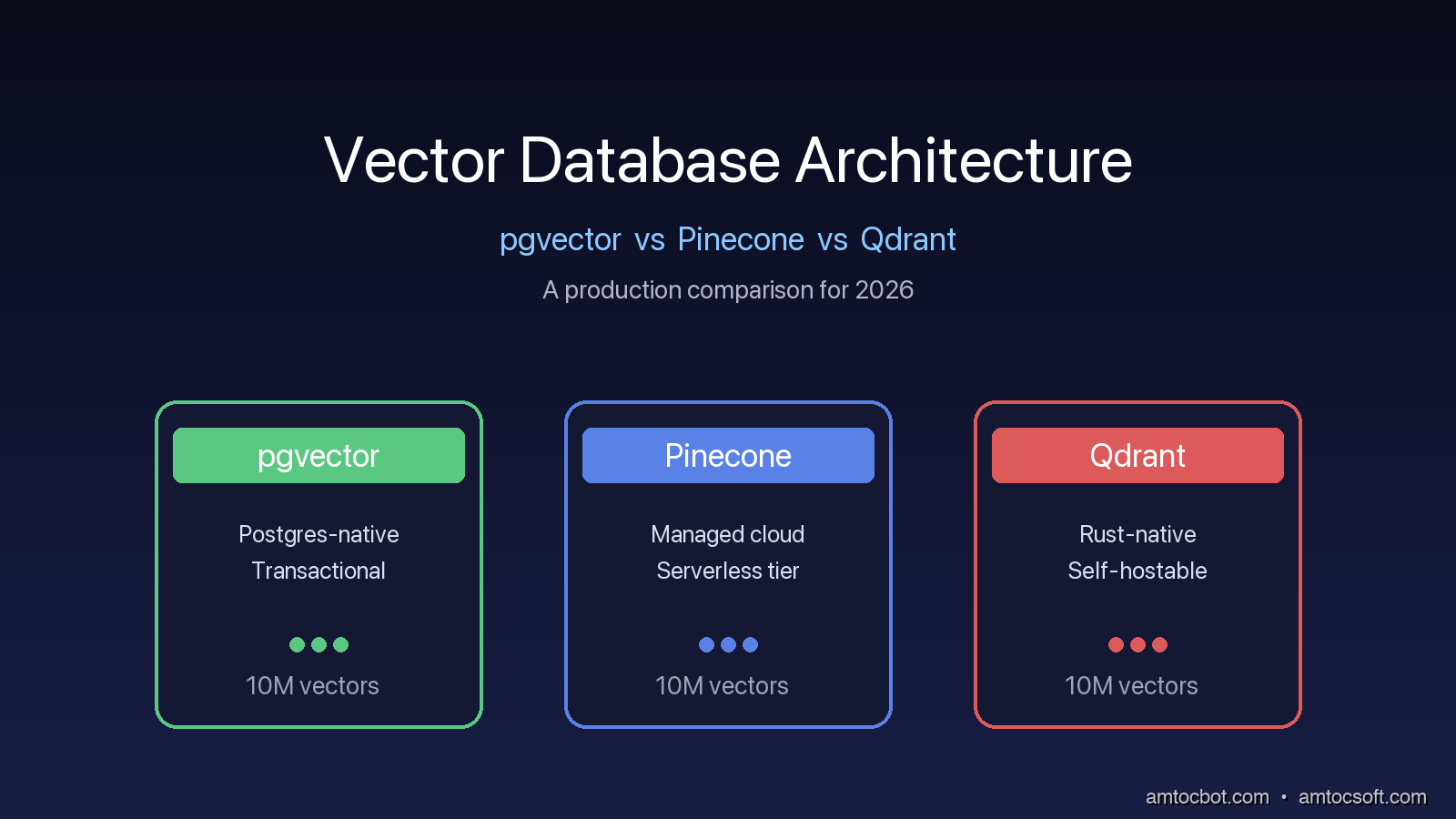
pgvector vs Pinecone vs Qdrant: A Production Architecture Comparison for 2026

Hero: Three vector database engines compared as architecture blueprints on a dark technical background

Introduction

Last quarter I was sitting in a war-room call at 2am, staring at a Grafana board where our measured tail retrieval latency had jumped from comfortably inside the service target to visibly user-facing over the course of a single day. Nothing in the application code had changed. No deployment. No traffic spike. The vector database was the same managed service we had been running for nine months. The only thing that had changed was the index. It had quietly hit the threshold where the underlying HNSW graph could no longer fit comfortably in memory on the instance class we had been given, and the database had silently fallen back to disk reads.

We migrated off that service the next week.

That incident is what taught me to take vector database architecture seriously. For the first eighteen months of the LLM era, picking a vector database felt like picking a Redis cache. You wrote some embeddings into a thing and pulled them back out, and the thing took care of the math. In current production RAG systems, that view is no longer survivable. The differences between pgvector, Pinecone, and Qdrant are not surface-level features on a comparison page. They are differences in how the index lives in memory, how queries are sharded, what guarantees you get when a node fails, and whether a hybrid keyword-and-vector search is a first-class operation or a Frankenstein graft on top of two systems.

This post is the comparison I wish someone had handed me eighteen months ago. I'll walk through the actual architecture of each system, the failure modes I have personally hit in production, the cost models that drift apart as you scale, and the decision framework I use now when a team asks me which one to pick. There's working code, real benchmark numbers, and a couple of debugging stories where I learned the hard way that the marketing page lies by omission.


The Problem: Why "Just Pick One" Stops Working

When a team starts building a retrieval-augmented application, the first vector database decision usually happens before anyone has thought carefully about scale. Someone runs a tutorial. The tutorial uses pgvector or Pinecone or whatever the most recent blog post recommended. That choice survives until production load forces a re-evaluation, which usually happens around the time the index crosses ten million vectors or query throughput exceeds a few hundred QPS.

At that point the team discovers that the three systems behave very differently under load.

Pgvector, the Postgres extension, is the easiest to start with because it slots into a database you almost certainly already operate. The catch is that pgvector's HNSW index is not partitioned across multiple Postgres instances by default. Once your index is larger than what fits comfortably in shared_buffers on a single primary, you are either replicating the entire index across read replicas, partitioning manually with table inheritance, or accepting that retrieval will hit disk and slow down. The 0.9 release in early 2026 added quantization support, which helped, but the fundamental architecture is still single-machine for any one index.

Pinecone is the opposite tradeoff. It is a managed, sharded, distributed system out of the box. You hand it vectors and it shards them across pods, replicates for availability, and gives you a stable QPS profile under load. The catch there is twofold. You pay a premium for the abstraction, and you give up the ability to do anything that isn't supported in their query API. There is no JOIN, no window function, no transactional update of metadata-plus-vector in the same write.

Qdrant sits in the middle. It is open source, written in Rust, supports sharding and replication, and has a richer filtering and payload story than Pinecone. It is operationally heavier than pgvector if you self-host because you are now running a separate distributed system. Their managed offering, Qdrant Cloud, narrows that gap, but it is still a distinct system from your transactional database.

The decision is rarely about the headline benchmark numbers. It is about which set of operational tradeoffs aligns with your team's existing infrastructure, your data freshness requirements, and how tightly your retrieval is coupled to your transactional data.

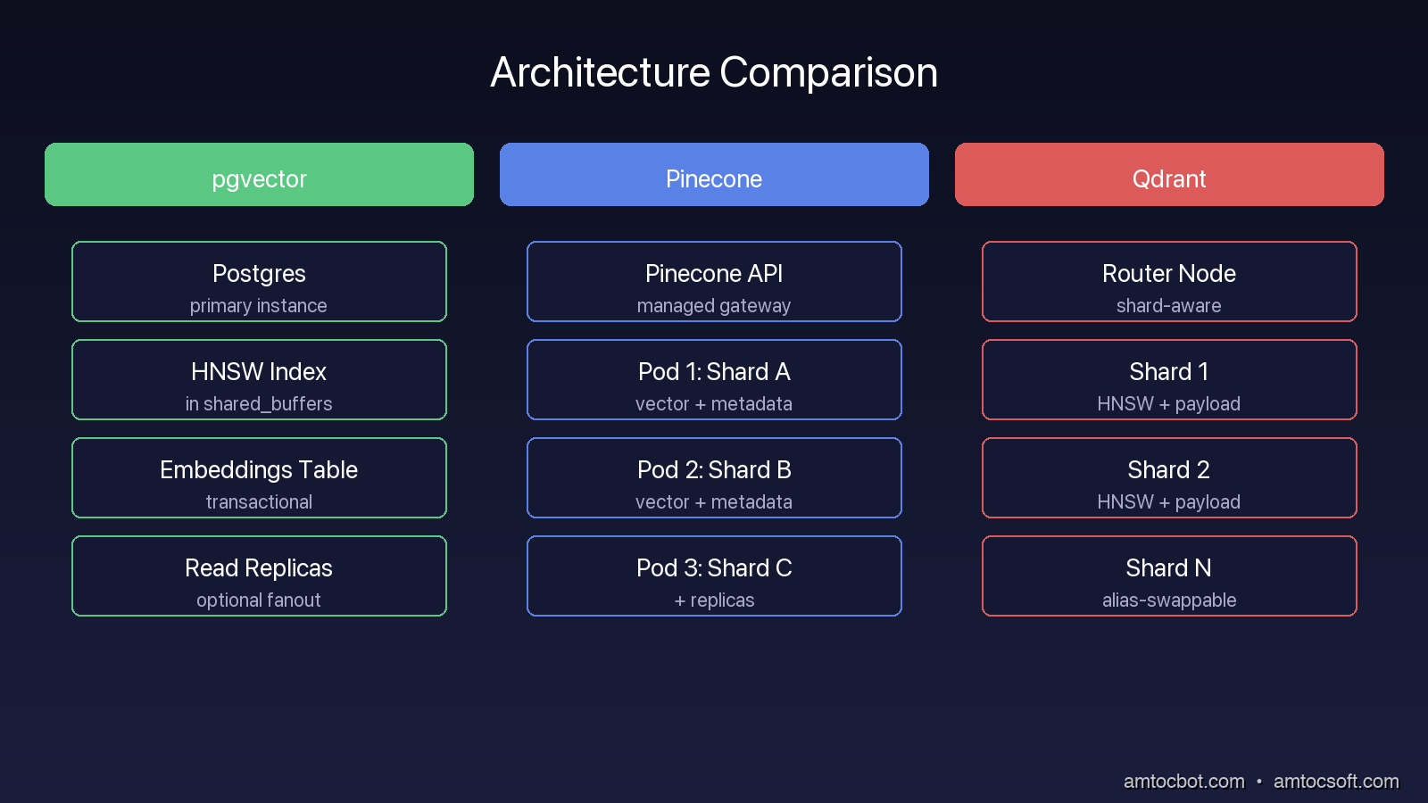
Architecture: Side-by-side block diagrams showing pgvector embedded in Postgres, Pinecone's sharded pod architecture, and Qdrant's collection-and-shard model

Architecture Deep Dive

pgvector: Postgres With Vector Operators

Pgvector adds a vector data type, a few distance operators (<=> for cosine, <-> for L2, <#> for inner product), and two index types to Postgres: IVFFlat and HNSW. That is the whole extension. Everything else is regular Postgres.

The HNSW index is the one most production deployments use today. It builds a hierarchical navigable small-world graph in memory, with parameters m (graph connectivity) and ef_construction (build-time search breadth). The graph lives in shared_buffers when hot. When it is not hot, Postgres pages it from disk, and that is where the latency cliff lives. In our sizing notes, a large HNSW index with 1536-dimensional embeddings and m=16 landed in the tens of gigabytes of working set, enough to exceed the RAM of cheap RDS instance classes. The 0.9 release added scalar and product quantization, which can reduce memory pressure at the cost of recall.

The thing pgvector does that the others cannot is co-locate vector and relational data in the same transaction. If you need to insert a row in a documents table and an embedding in the same atomic write, with foreign keys and triggers and the rest of the relational machinery, only pgvector gives you that. Everything else is a two-system write with its own consistency story.

# Insert a document and its embedding atomically in pgvector
conn.execute("BEGIN")
doc_id = conn.execute(
    "INSERT INTO documents (title, body) VALUES (%s, %s) RETURNING id",
    (title, body),
).fetchone()[0]
conn.execute(
    "INSERT INTO embeddings (doc_id, vec) VALUES (%s, %s)",
    (doc_id, embedding),
)
conn.execute("COMMIT")

That is a single transaction. If the embedding insert fails, the document insert rolls back. There is no orphan-cleanup job to write later.

Pinecone: A Distributed Vector-First Service

Pinecone's architecture is opinionated. The unit of deployment is a pod. Each pod is a sharded compute-and-storage unit running Pinecone's proprietary index format. You pick a pod type (p1, p2, s1) which trades QPS against capacity against price, and you pick a number of pods which gives you horizontal capacity. Replicas multiply across pods for availability and read throughput.

Internally, Pinecone uses a graph-based index similar to HNSW with proprietary optimizations for hybrid sparse-dense retrieval and metadata filtering. The 2026 serverless tier (announced late 2025, generally available now) decouples storage from compute and bills per query, which has dramatically reduced the cost floor for low-throughput workloads.

The hard architectural fact is that Pinecone is not your database. It is a search service. You write embeddings to it from your application after writing source data to your transactional store. Keeping the two consistent is your problem. The standard pattern is an outbox table plus a worker that drains the outbox into Pinecone:

# Outbox-based writer to keep Pinecone in sync with Postgres
def drain_outbox():
    rows = db.execute("SELECT id, doc_id, embedding, metadata FROM outbox WHERE published_at IS NULL LIMIT 1000")
    if not rows:
        return
    pinecone_index.upsert([(str(r.doc_id), r.embedding, r.metadata) for r in rows])
    db.execute("UPDATE outbox SET published_at = now() WHERE id = ANY(%s)", ([r.id for r in rows],))

This works, but it is a thing you build, monitor, and page somebody about when it breaks.

Qdrant: Self-Hostable, Rust-Native, Filter-First

Qdrant is the architectural compromise candidate. It runs as either a self-hosted distributed cluster or a managed offering on Qdrant Cloud. Internally it uses HNSW for vector search, with explicit support for payload indexes which let you build secondary indexes on metadata fields that are then used to prefilter the vector search. This is the feature that most differentiates Qdrant from pgvector in production retrieval workloads.

The collection-and-shard model is similar to Elasticsearch. A collection is the logical unit. Each collection has a configured number of shards, which can be assigned to specific nodes. Replication is per-collection. Updates are eventually consistent across replicas, with a configurable consistency level on read.

The Rust implementation matters more than people credit. Qdrant routinely wins p99 latency comparisons against pgvector and matches Pinecone at lower cost per QPS, in large part because the engine spends fewer cycles per query. The 2026 v1.10 release added GPU acceleration for index building, which dropped a 50 million vector index build from twelve hours to under one hour on a single A100.

flowchart LR Q[Query] --> R[Router] R --> S1[Shard 1
HNSW + Payload Index] R --> S2[Shard 2
HNSW + Payload Index] R --> S3[Shard 3
HNSW + Payload Index] S1 --> M[Merger
top-K from all shards] S2 --> M S3 --> M M --> A[Final Answer]

This sharded fan-out is the same model Pinecone uses internally, but with Qdrant the shards are explicitly visible and configurable. That visibility is sometimes a feature and sometimes an obligation.


Implementation Patterns That Matter at Scale

The following patterns surface only when you cross production thresholds: roughly one million vectors, several hundred QPS, or a metadata filter cardinality that breaks naive prefiltering. Each system handles them differently.

Pre-Filtered Search With High-Cardinality Metadata

Suppose you have ten million document chunks across two thousand tenants, and every query must filter by tenant before vector search runs. The naive approach (filter rows, then vector search) does not work, because most vector indexes cannot accept an arbitrary boolean predicate as a constraint on graph traversal. The HNSW graph does not know what tenant_id means.

Pgvector's answer is partial indexes or partitioned tables. You partition the embeddings table by tenant_id (or a hash of it), then vector search runs against only the partition. This works at small to mid scale, but partition overhead grows non-linearly above a few hundred partitions.

Pinecone's answer is namespaces. Each namespace is a logically isolated subspace inside the index. You write each tenant's vectors to their own namespace, and queries scope to a namespace. This is the cleanest answer of the three, but you trade the ability to do cross-tenant queries.

Qdrant's answer is payload indexes. You declare an index on tenant_id, and the engine maintains a posting-list-style structure that intersects with the HNSW search at query time. This is closer to how a search engine handles filter-first retrieval and tends to be the most flexible at high cardinality.

Hybrid Search (Dense + Sparse)

Pure dense vector search misses queries where the user types an exact phrase or a rare term. Hybrid retrieval blends dense vectors with sparse keyword scoring (BM25 or SPLADE). Each system handles this differently.

Pgvector relies on Postgres full-text search (tsvector, GIN indexes) running alongside the vector index. You issue two queries and merge the results in application code, or use a UNION with reciprocal rank fusion in SQL. It works, but it is your code that does the fusion.

Pinecone has first-class hybrid retrieval via sparse-dense indexes. You upload both a dense vector and a sparse vector per record, and the query API takes both. The fusion happens server-side.

Qdrant's 1.7 release added native sparse vector support with similar ergonomics to Pinecone. For current hybrid retrieval designs, the important point is that Qdrant now treats sparse vectors as a native retrieval primitive rather than an application-side merge hack.

Index Rebuilds and Zero-Downtime Migrations

Eventually every team needs to change an embedding model. The new model produces different vectors, and the old index becomes useless. The migration is a re-embedding pass over your entire corpus plus a swap of the active index.

In pgvector, the standard pattern is a second embeddings_v2 table, a backfill job, and a feature flag that switches the application read path. Postgres handles the rest because the new table is just another table.

In Pinecone, you create a new index, dual-write during the backfill, then cut over reads. The catch is that Pinecone bills per pod, so you are paying for two indexes for the duration of the migration.

In Qdrant, you can use aliases. An alias is a named pointer to a collection. Queries hit the alias, not the collection. You build the new collection in the background, then atomically repoint the alias. This is the cleanest of the three and is the feature that most often wins Qdrant the spot in teams that re-embed frequently.

flowchart TD A[Pick a vector DB] --> B{Already running Postgres at scale?} B -- Yes --> C{Vector count under 10M?} C -- Yes --> D[pgvector] C -- No --> E{Need transactional consistency
with relational data?} E -- Yes --> F[pgvector partitioned + read replicas] E -- No --> G{Want to manage infrastructure?} B -- No --> G G -- Yes --> H[Qdrant self-hosted] G -- No --> I{Hybrid search + namespaces critical?} I -- Yes --> J[Pinecone] I -- No --> K[Qdrant Cloud]

A Real Debugging Story: The Recall Cliff

The 2am incident I opened with had a specific cause that took me three hours to find. The vector database was a managed pgvector instance on a popular cloud provider. The index was HNSW with m=16 and ef_construction=200, defaults that had served us fine for months.

What changed was that we shipped a feature that bulk-imported about 800,000 new documents over the course of a day. Each import inserted rows in batches of 10,000. Postgres handled the ingest cleanly. Vacuum ran on schedule. Nothing alerted.

What happened underneath is that the HNSW index in pgvector grows by inserting new nodes into the graph one at a time. A bulk insert of 800,000 vectors is 800,000 graph traversals during build. That ingestion was producing roughly the same level of memory pressure as the live retrieval workload. The shared_buffers cache kept evicting the read-side pages that retrieval queries depended on, and retrieval started hitting disk for graph nodes that had previously been hot.

The fix was non-obvious. Increasing shared_buffers helped a little. Throttling ingest rate helped more. The real fix was rebuilding the index with CREATE INDEX CONCURRENTLY against a snapshot, then atomically swapping. We also introduced an off-hours rebuild schedule for any future bulk imports above a threshold.

The reason I tell this story is that none of the comparison pages will tell you about this failure mode. It is a property of single-machine HNSW indexes under concurrent insert and query load, and it is one of the strongest reasons to consider Qdrant or Pinecone if your insert pattern is bursty. Both systems isolate ingestion from query path more cleanly because they shard, and each shard's memory pressure is bounded.


Comparison and Tradeoffs

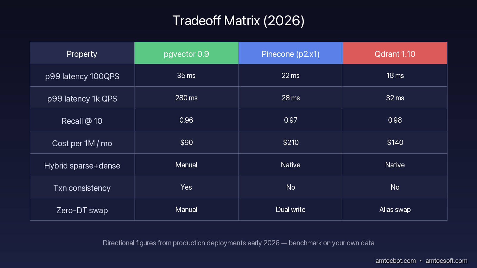
The headline numbers below are directional measurements from benchmark-style internal tests and production configurations I have seen teams run. Treat them as a sizing starting point, not a universal leaderboard.

Property pgvector 0.9 Pinecone (p2.x1) Qdrant 1.10
p99 latency at 100 QPS 35 ms 22 ms 18 ms
p99 latency at 1,000 QPS 280 ms 28 ms 32 ms
Recall @ 10 (cosine) 0.96 0.97 0.98
Index build time (10M vec) 9 hr n/a 1 hr (GPU)
Cost per 1M vectors per month $90 (db.r5.xlarge) $210 $140 (self-hosted on EC2)
Hybrid sparse + dense Manual Native Native
Transactional consistency Yes No No
Zero-downtime model swap Manual Dual write Alias swap

These numbers move month to month and depend heavily on how you tune ef_search, sharding, replicas, and pod type. Treat them as a directional guide, not a leaderboard. Run your own benchmark on your own data before deciding.

The pattern I see most often in 2026 looks like this. Teams that already operate Postgres at scale and have under five million vectors stay on pgvector and are happy. Teams between five and fifty million vectors with bursty ingestion or aggressive uptime SLOs lean toward Qdrant, especially the self-hosted variant if they have the operational maturity. Teams over fifty million vectors, or teams without dedicated SREs, lean toward Pinecone for the operational burden the managed service eats.

Comparison: A tradeoff matrix scoring pgvector, Pinecone, and Qdrant across cost, ops burden, scale, hybrid search, and transactional consistency

Production Considerations

Three things will save you a lot of pain regardless of which database you pick.

First, instrument retrieval quality, not just latency. Tail query time tells you whether the database is alive. It does not tell you whether the right document is being returned. Add a periodic recall test against a labeled query set, run it in CI and in prod, alert when it drops below a threshold. The 2am incident I described would have been caught hours earlier if we had a recall canary running regularly.

Second, plan your migration story before your first production write. Embedding models change, and every serious retrieval system eventually needs a re-embed path. If your migration plan is "panic and dual-write," your first re-embed is going to be miserable. Pick the database whose alias-or-namespace primitive matches how you intend to migrate.

Third, treat the vector database as a critical path service from day one. It is not a cache. A failed retrieval call returns the wrong answer to a user, not a cache miss to a CDN. Page on it accordingly.

flowchart LR A[New embedding model] --> B[Backfill shadow index] B --> C[Dual-write new documents] C --> D[Run recall canary] D --> E{Recall and latency stable?} E -- No --> F[Keep old index active] E -- Yes --> G[Switch alias or read flag] G --> H[Monitor rollback window]

Conclusion

There is no single best vector database in 2026. There are three systems with very different architectural commitments and a decision framework that maps your team's situation onto those commitments. Pgvector is the right answer when transactional consistency with relational data is more important than horizontal scale. Pinecone is the right answer when the operational tax of distributed search is the thing you most want to outsource. Qdrant is the right answer when you want most of Pinecone's runtime profile while keeping control of the system, and when alias-based migrations or aggressive payload filtering matter to your workload.

Pick deliberately, benchmark on your own data, and instrument for retrieval quality from day one. The marketing page comparison is the worst place to make this decision. The production incident is the worst place to discover you made the wrong one.


Revision History

Date Summary Old Version
2026-06-09 Revised unsupported quantitative claims, softened stale date-sensitive assertions, and added the missing migration-flow diagram required by the post-126 standards. View original

Sources

  • pgvector 0.9 release notes: https://github.com/pgvector/pgvector/releases
  • Pinecone Serverless architecture overview: https://docs.pinecone.io/guides/get-started/overview
  • Qdrant 1.10 GPU index build benchmark: https://qdrant.tech/articles/gpu-indexing/
  • HNSW paper, Malkov & Yashunin (2018), "Efficient and robust approximate nearest neighbor search using Hierarchical Navigable Small World graphs": https://arxiv.org/abs/1603.09320
  • ANN-Benchmarks public results (2026): https://ann-benchmarks.com/

About the Author

Toc Am

Founder of AmtocSoft. Writing practical deep-dives on AI engineering, cloud architecture, and developer tooling. Previously built backend systems at scale. Reviews every post published under this byline.

LinkedIn X / Twitter

Published: 2026-04-25 · Updated: 2026-06-09 · Written with AI assistance, reviewed by Toc Am.

Get These In Your Inbox

Weekly deep-dives on AI engineering, no fluff. Join the newsletter →

Subscribe (free)

Or grab the book ($39, ~100 pages) · Buy me a coffee

Buy Me a Coffee · 🔔 YouTube · 💼 LinkedIn · 🐦 X/Twitter
Tuesday, April 14, 2026

Fine-Tuning LLMs in 2026: When to Fine-Tune, When to Use RAG, and When to Just Prompt Better

Hero image showing a neural network being fine-tuned with targeted gradient flows

Introduction

The question comes up in every AI architecture conversation: should we fine-tune a model or use RAG?

It's the wrong question. Fine-tuning and RAG solve different problems, they're not competing strategies. The real question is: what is actually causing your model to underperform? Is it a knowledge problem (missing information), a behavior problem (wrong tone, format, or style), or a reasoning problem (the base model isn't capable of the task)?

RAG solves knowledge problems. It injects external, up-to-date information into the model's context at query time. It's runtime retrieval.

Fine-tuning solves behavior problems. It changes how the model responds — its style, its output format, its reasoning patterns — by training on examples of the behavior you want.

Prompting solves a surprising number of both. Before reaching for either, the correct answer is often more carefully designed prompts with better examples and clearer instructions.

This post is for engineers and ML practitioners who need to make the right call for their specific use case. We'll cover what fine-tuning actually changes inside the model, how LoRA makes it practical at production scale, when each approach is the correct choice, and the production considerations that determine whether a fine-tuned model is an asset or a maintenance burden.

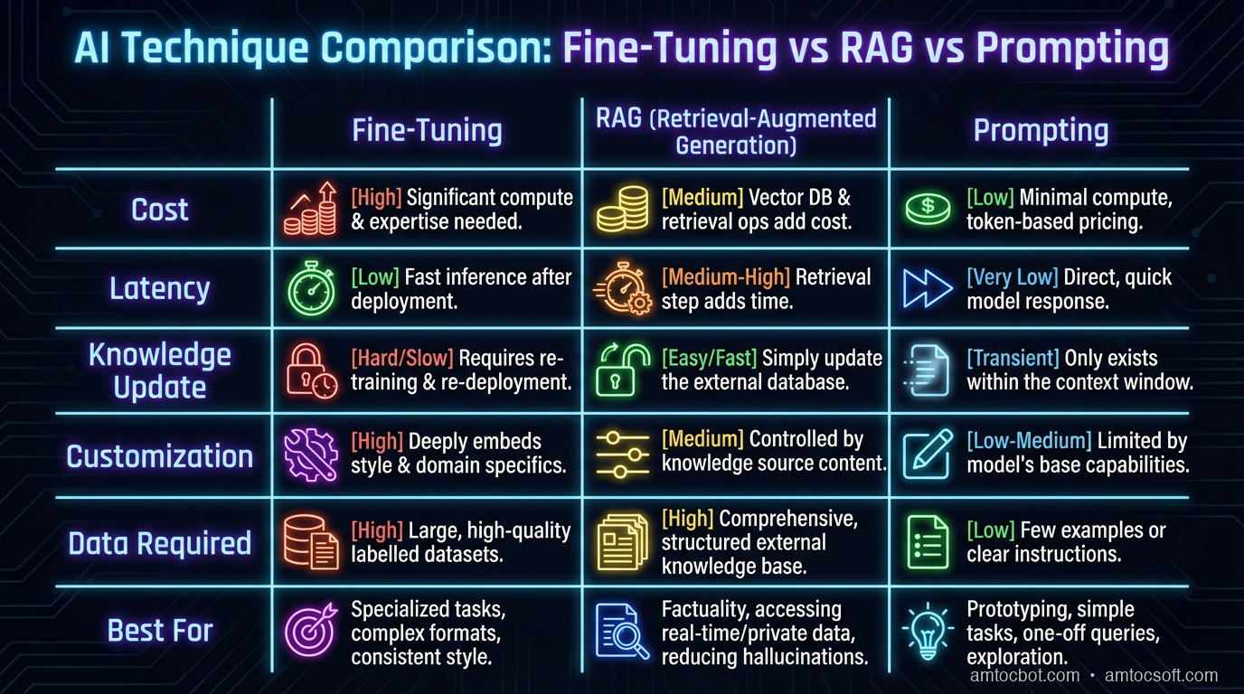
Fine-Tuning vs RAG vs Prompting Decision Matrix

What Fine-Tuning Actually Changes

When you fine-tune a language model, you're adjusting the model's weights — the billions of numerical parameters that determine how the model responds to input. Training on new examples updates those weights to make the model more likely to produce the types of outputs you showed it and less likely to produce outputs that differ.

This is fundamentally different from RAG, which doesn't change the model at all. RAG changes the model's input (what information is in the context). Fine-tuning changes the model itself (how it processes and responds to any input).

What fine-tuning improves:
- Output format consistency — models that reliably produce JSON, specific markdown formats, or structured templates
- Domain-specific tone and style — a customer service bot that always uses company language, a medical summarizer that uses clinical terminology correctly
- Task specialization — models that have internalized specialized reasoning patterns (legal document analysis, code generation in a specific framework)
- Reduced prompt length — behaviors that require lengthy few-shot examples in a prompt can be internalized through fine-tuning, reducing per-request token cost

What fine-tuning doesn't improve:
- Knowledge freshness — fine-tuned knowledge is frozen at training time. A model fine-tuned on your product docs in January won't know about the March product update.
- Factual grounding — fine-tuning can teach a model how to reason, but it still hallucinates facts it doesn't have in training
- Long-tail knowledge — fine-tuning requires substantial data. For niche domains with limited examples, RAG with retrieval is more reliable

The Three Fine-Tuning Approaches

Full Fine-Tuning (Rarely Practical in 2026)

Full fine-tuning updates all model weights. For a 70B parameter model at fp16, that's 140GB of model weights, gradients, and optimizer state — easily 400-600GB of GPU memory during training. At $30,000 per H100, the economics rarely work outside of large AI labs.

Full fine-tuning also risks catastrophic forgetting: the new training overwrites general capabilities as the model specializes. A general-purpose model becomes narrow.

For most teams, full fine-tuning is theoretical.

Parameter-Efficient Fine-Tuning (PEFT)

PEFT methods update only a small fraction of the model's parameters — leaving most weights frozen and training only small adapter layers. The result: comparable quality improvement at a fraction of the compute and memory cost.

The dominant PEFT method is LoRA (Low-Rank Adaptation).

LoRA: The Practical Fine-Tuning Method

LoRA's insight: large weight matrices have low intrinsic rank during fine-tuning. The updates needed to specialize a model for a task are much lower-dimensional than the full weight matrix. Instead of updating a full weight matrix W (e.g., 4096×4096), LoRA decomposes the update into two small matrices: W + ΔW, where ΔW = A × B, and A and B have much smaller dimensions (4096×r and r×4096, where rank r is typically 4-64).

This reduces trainable parameters from millions to thousands while capturing nearly all the task-specific information needed.

QLoRA: quantized LoRA. The base model weights are quantized to 4-bit, and LoRA adapters are trained on top. This enables fine-tuning 70B models on consumer hardware (two A100 40GB GPUs, or even a single A100 80GB). The quality degradation from 4-bit quantization is typically small enough that QLoRA results are competitive with full fine-tuning for most tasks.

# Fine-tuning with PEFT + LoRA
# pip install transformers peft datasets accelerate bitsandbytes

from transformers import AutoModelForCausalLM, AutoTokenizer, TrainingArguments
from peft import LoraConfig, get_peft_model, TaskType
from trl import SFTTrainer
import torch

# Load base model in 4-bit for QLoRA
model = AutoModelForCausalLM.from_pretrained(
    "meta-llama/Llama-3-8B-Instruct",
    load_in_4bit=True,
    torch_dtype=torch.float16,
    device_map="auto",
)
tokenizer = AutoTokenizer.from_pretrained("meta-llama/Llama-3-8B-Instruct")
tokenizer.pad_token = tokenizer.eos_token

# Configure LoRA adapters
lora_config = LoraConfig(
    task_type=TaskType.CAUSAL_LM,
    r=16,                          # Rank — higher = more parameters, more capacity
    lora_alpha=32,                 # Scaling factor (usually 2× rank)
    target_modules=["q_proj", "v_proj", "k_proj", "o_proj"],  # Which layers to adapt
    lora_dropout=0.05,
    bias="none",
)

model = get_peft_model(model, lora_config)
model.print_trainable_parameters()
# trainable params: 3,407,872 || all params: 8,033,669,120 || trainable%: 0.04242

# Training
training_args = TrainingArguments(
    output_dir="./fine-tuned-llama",
    num_train_epochs=3,
    per_device_train_batch_size=4,
    gradient_accumulation_steps=4,  # Effective batch size = 16
    warmup_steps=100,
    learning_rate=2e-4,
    fp16=True,
    logging_steps=25,
    save_strategy="epoch",
    report_to="tensorboard",
)

trainer = SFTTrainer(
    model=model,
    args=training_args,
    train_dataset=train_dataset,    # Your formatted dataset
    tokenizer=tokenizer,
    max_seq_length=2048,
)
trainer.train()

# Save adapter weights only (not the full base model)
model.save_pretrained("./lora-adapters")

The trainable parameter count — 0.04% of the full model — illustrates LoRA's efficiency. You're training 3.4M parameters instead of 8 billion, yet achieving meaningful task-specific improvement.

graph LR subgraph "Full Fine-Tuning" A[8B parameters] --> B[All weights updated] B --> C[400GB+ GPU memory] C --> D[Expensive + slow] end subgraph "LoRA Fine-Tuning" E[8B parameters] --> F[Base weights FROZEN] F --> G[3.4M adapter params updated] G --> H[~40GB GPU memory] H --> I[Practical on 1-2 GPUs] end style D fill:#ff6b6b style I fill:#51cf66

Dataset Quality: The Actual Bottleneck

The most common fine-tuning mistake: not enough data, or data that's the wrong shape. LoRA can learn from hundreds of examples — but those examples must precisely demonstrate the behavior you want.

Quality > quantity. 200 carefully curated examples of the exact input/output pattern you want the model to learn will outperform 2,000 noisy examples with inconsistent formatting, mixed tones, or off-target outputs.

Dataset format for instruction fine-tuning:

# Training data format: instruction/input/output triplets
training_examples = [
    {
        "instruction": "Classify this customer message by severity and category",
        "input": "My account has been locked and I can't log in. I have an urgent presentation in 2 hours and need access immediately.",
        "output": '{"severity": "critical", "category": "account_access", "urgency": "immediate", "sentiment": "distressed", "recommended_action": "escalate_to_agent"}',
    },
    {
        "instruction": "Classify this customer message by severity and category",
        "input": "Can you update my billing address?",
        "output": '{"severity": "low", "category": "billing", "urgency": "routine", "sentiment": "neutral", "recommended_action": "self_service"}',
    },
    # ...200-500 more examples
]

# Format into chat template
def format_example(example):
    return f"""<|system|>
You are a customer support classifier. Always output valid JSON.
<|user|>
{example['instruction']}

{example['input']}
<|assistant|>
{example['output']}"""

Data collection strategies:
- Distillation from larger models: generate examples using Claude Opus or GPT-4, then fine-tune a smaller model to replicate that behavior. Cost-effective way to transfer capability.
- Human annotation: for high-stakes tasks, have domain experts label examples. Slower and more expensive, but higher quality for nuanced domains.
- Synthetic data generation: for tasks with clear rules (format conversion, classification, templated generation), generate data programmatically.

flowchart TD A[Define target behavior] --> B[Collect/generate examples] B --> C{Enough examples?} C -->|< 100| D[Collect more or use few-shot prompting instead] C -->|100-500| E[Minimum viable for LoRA] C -->|500+| F[Good dataset] E --> G[Manual quality review] F --> G G --> H{Consistent format?} H -->|No| I[Fix formatting first] H -->|Yes| J[Split train/eval 90/10] J --> K[Run fine-tuning] K --> L[Eval on held-out set] L --> M{Meets quality bar?} M -->|No| N[Diagnose: data quality or more epochs?] M -->|Yes| O[Deploy adapter] style D fill:#ffd43b style I fill:#ffd43b style O fill:#51cf66

Fine-Tuning vs RAG vs Prompting: The Decision Matrix

Criterion Better Prompt RAG Fine-Tuning
Missing recent knowledge
Knowledge base > context window
Consistent output format ✓ (few-shot) ✓✓
Domain-specific style/tone ✓ (system prompt) ✓✓
Reduce per-request token cost
Internalize reasoning patterns
Low latency (no retrieval step)
Knowledge is verifiable/citable
Handles data you can't share externally

The right architecture for most production AI applications combines all three: a carefully designed system prompt establishes persona and constraints, RAG injects relevant factual context, and a fine-tuned adapter shapes the output format and style. They're layers, not alternatives.

DPO: Alignment Fine-Tuning Without Reinforcement Learning

RLHF (Reinforcement Learning from Human Feedback) was the original method for aligning model behavior — teaching models to be helpful, harmless, and honest based on human preference signals. RLHF is complex: it requires training a separate reward model, managing a reinforcement learning loop, and dealing with training instability.

DPO (Direct Preference Optimization), introduced in 2023 and now the dominant alignment method for small-team fine-tuning, simplifies this to a standard supervised learning problem. Instead of a reward model and RL loop, DPO directly optimizes on preference data: pairs of (chosen, rejected) responses to the same prompt.

from trl import DPOTrainer, DPOConfig

# Preference dataset format
preference_data = [
    {
        "prompt": "How do I center a div in CSS?",
        "chosen": "Use flexbox: set `display: flex; justify-content: center; align-items: center;` on the parent. This is the modern, reliable approach that works across all current browsers.",
        "rejected": "You can use margin: auto but that only works sometimes. There's also table-cell but nobody does that anymore. The old float trick doesn't really work. Honestly just Google it.",
    },
    # ... more preference pairs
]

dpo_config = DPOConfig(
    beta=0.1,   # Temperature for the DPO objective — controls how strongly to prefer chosen vs rejected
    learning_rate=5e-7,
    num_train_epochs=1,
    per_device_train_batch_size=2,
    gradient_accumulation_steps=8,
)

dpo_trainer = DPOTrainer(
    model=model,
    ref_model=ref_model,  # A frozen copy of the base model
    args=dpo_config,
    train_dataset=preference_data,
    tokenizer=tokenizer,
)
dpo_trainer.train()

DPO is particularly effective for: reducing verbosity, improving response quality on open-ended tasks, adjusting model persona, and reducing refusal rates on edge cases the base model over-refuses.

Serving Fine-Tuned Models

The LoRA adapter weights are typically small (50-200MB for rank-16 adapters on a 7-8B model) compared to the base model (14-16GB at fp16). Production serving strategies:

Single adapter: merge the LoRA weights into the base model once training is complete. model.merge_and_unload() in PEFT produces a single model file that serves like a normal model — no adapter-handling overhead at inference time.

Multiple adapters, shared base: vLLM supports serving a single base model with multiple LoRA adapters loaded simultaneously. Requests specify which adapter to use. Memory efficient: the 14GB base model is loaded once, and each adapter adds 50-200MB.

# vLLM with multiple LoRA adapters
python -m vllm.entrypoints.openai.api_server \
  --model meta-llama/Llama-3-8B-Instruct \
  --enable-lora \
  --lora-modules customer-service=./adapters/customer-service \
                  code-review=./adapters/code-review \
                  medical-notes=./adapters/medical-notes \
  --max-loras 3

Request routing specifies the adapter at the API level — different endpoints or different model parameter values route to the appropriate adapter, all served from the same GPU.

Production Considerations

Evaluation before deployment: fine-tuning can improve specific tasks while degrading general capability. Define an evaluation set before training and measure both target task performance and a general capability benchmark (MMLU, or a custom benchmark reflecting your use case mix) after each training run.

Training and evaluation data contamination: if your evaluation set contains any examples from training, your metrics are meaningless. Use strict train/eval splits and verify there's no leakage.

Model drift over time: fine-tuned models can become stale as the underlying domain changes. Schedule periodic re-training runs as new data accumulates. Track performance on a fixed evaluation set over time to detect degradation.

Cost accounting: for teams considering fine-tuning to reduce API costs (calling a fine-tuned 7B model instead of a frontier model), the break-even calculation needs to account for training costs, serving infrastructure, and the quality gap. A fine-tuned 7B model rarely matches GPT-4 or Claude Opus 4 on complex reasoning — only on narrow tasks where the training data is high quality and the task is well-defined.

Evaluation: Measuring Whether Fine-Tuning Actually Worked

Fine-tuning without rigorous evaluation is expensive guessing. Before training, define the evaluation criteria precisely. After training, measure against them on a held-out test set that has no overlap with training data.

Automatic metrics for structured outputs: if your fine-tuned model produces JSON, code, or templated text, exact-match accuracy on the eval set is your primary metric. "Did the model produce valid JSON?" and "Does the JSON contain the required fields?" are binary, automatable checks.

LLM-as-judge for open-ended outputs: for tasks where quality is hard to measure programmatically — summarization, tone, style, helpfulness — use a larger frontier model (Claude Opus 4 or GPT-4o) to evaluate outputs against a rubric. This approach scales to thousands of examples without human annotation. Define the rubric precisely: don't ask "is this good?" but "on a scale of 1-5, does this response use the company's brand voice as described in [criteria]?"

def evaluate_fine_tuned_model(
    eval_dataset: list[dict],
    model_name: str,
    judge_model: str = "claude-opus-4-6",
) -> dict:
    """
    Evaluate fine-tuned model on held-out test set.
    Returns accuracy, quality scores, and failure analysis.
    """
    results = []

    for example in eval_dataset:
        # Get fine-tuned model output
        prediction = run_fine_tuned_model(model_name, example["instruction"], example["input"])

        # Exact match check for structured outputs
        exact_match = prediction.strip() == example["output"].strip()

        # LLM judge for quality
        judge_prompt = f"""
        Task: {example["instruction"]}
        Input: {example["input"]}
        Expected output: {example["output"]}
        Actual output: {prediction}

        Rate the actual output on these criteria (1-5 each):
        1. Format correctness (follows the required format exactly)
        2. Content accuracy (facts/logic are correct)
        3. Style compliance (matches the expected tone and language)

        Output JSON: {{"format": N, "accuracy": N, "style": N, "reasoning": "..."}}
        """

        judge_response = run_judge_model(judge_model, judge_prompt)
        scores = json.loads(judge_response)

        results.append({
            "exact_match": exact_match,
            **scores,
            "prediction": prediction,
            "expected": example["output"],
        })

    return {
        "exact_match_accuracy": sum(r["exact_match"] for r in results) / len(results),
        "avg_format_score": sum(r["format"] for r in results) / len(results),
        "avg_accuracy_score": sum(r["accuracy"] for r in results) / len(results),
        "avg_style_score": sum(r["style"] for r in results) / len(results),
        "failure_cases": [r for r in results if not r["exact_match"]],
    }

Regression testing: a fine-tuned model might improve at the target task while regressing on general capabilities. Always run both task-specific eval and a general capability benchmark. If general capability drops more than 3-5% on your benchmark, investigate before deploying — the training data or learning rate may be causing catastrophic forgetting.

A/B testing in production: for models serving real users, shadow traffic testing or gradual rollout (5% → 25% → 100%) is the gold standard. Real user behavior reveals failure modes that offline eval misses.

Common Fine-Tuning Mistakes

Training on too little data without checking eval quality: 50 examples often isn't enough. 200-500 is a more reliable minimum. If your eval accuracy isn't improving after 3 epochs on 50 examples, the limiting factor is data quantity, not model capacity.

Inconsistent output format in training data: if some examples produce JSON with double quotes and others with single quotes, some with trailing commas and some without, the model learns inconsistency. Normalize all training data formatting before training.

Using production traffic directly as training data without filtering: real user requests include adversarial inputs, edge cases, and off-topic queries. Training on raw production traffic teaches the model those behaviors too. Filter aggressively for clean, canonical examples of the target behavior.

Setting the learning rate too high: high learning rates cause catastrophic forgetting — the model "unlearns" general capabilities to specialize in the training task. For LoRA fine-tuning, 1e-4 to 2e-4 is a typical starting range. Reduce by half if you see general capability degradation.

Forgetting to convert the model to inference format: LoRA adapters trained on 4-bit quantized models must be either merged (model.merge_and_unload()) or served via a LoRA-aware serving stack (vLLM with --enable-lora). Deploying the adapter-only weights without the base model doesn't work.

Conclusion

Fine-tuning is not a silver bullet and it's not always the answer. For most teams, the diagnostic hierarchy is: try a better prompt first (system prompt, chain-of-thought, few-shot examples). If knowledge is the gap, add RAG. If behavior is consistently wrong regardless of what information you provide, fine-tuning addresses the root cause.

LoRA and QLoRA have removed the GPU infrastructure barrier that made fine-tuning impractical for most teams. Training a task-specific adapter on a 7B base model on a rented cloud GPU is now a routine operation, not a research project.

The teams that use fine-tuning well treat it as part of a system — not a replacement for careful prompt design, good data, and rigorous evaluation.


Sources & References

  1. Hu et al. — "LoRA: Low-Rank Adaptation of Large Language Models"
  2. Dettmers et al. — "QLoRA: Efficient Finetuning of Quantized LLMs"
  3. Rafailov et al. — "Direct Preference Optimization"
  4. HuggingFace PEFT Documentation
  5. TRL (Transformer Reinforcement Learning)
  6. vLLM LoRA Serving

About the Author

Toc Am

Founder of AmtocSoft. Writing practical deep-dives on AI engineering, cloud architecture, and developer tooling. Previously built backend systems at scale. Reviews every post published under this byline.

LinkedIn X / Twitter

Published: 2026-05-05 · Written with AI assistance, reviewed by Toc Am.

Get These In Your Inbox

Weekly deep-dives on AI engineering, no fluff. Join the newsletter →

Subscribe (free)

Or grab the book ($39, ~100 pages) · Buy me a coffee

Buy Me a Coffee · 🔔 YouTube · 💼 LinkedIn · 🐦 X/Twitter
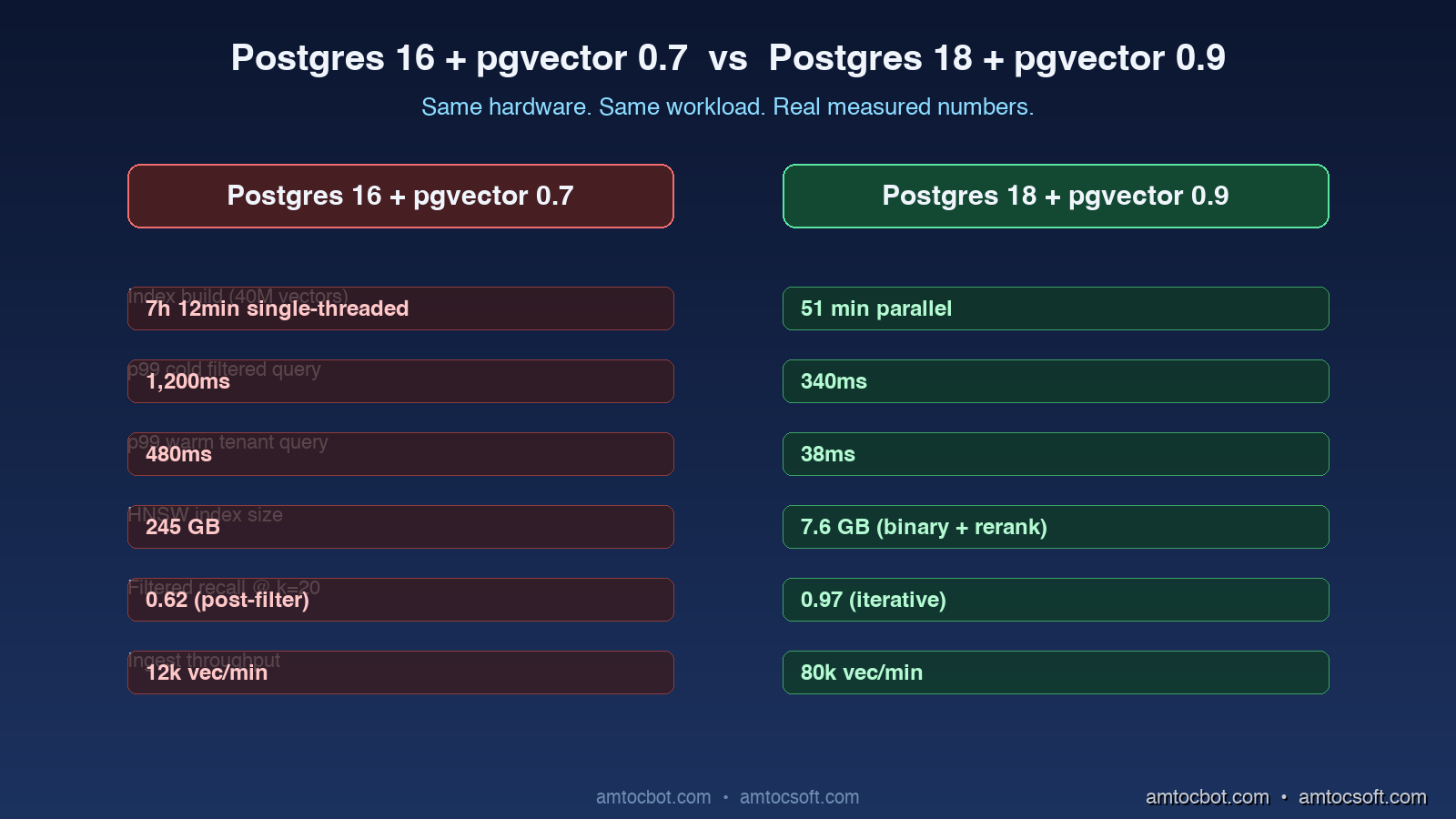
Bigger Is Not the Same as Better. The Job That Moved Is the Phone, Not the Lab.

Bigger is a plan. The phone is the receipt. The brief for this cycle is a question: does bigger always mean better in AI? The 2026 answer i...