Showing posts with label prompt-caching. Show all posts

Wednesday, July 1, 2026

Prompt Caching in Production: How to Structure LLM Calls to Cut Inference Costs by 80%

Hero: glowing server rack with cache hit indicators and cost charts falling

Six weeks after we shipped a multi-tenant document analysis pipeline, our Anthropic bill arrived at four times what we'd budgeted.

The pipeline was working correctly. Response quality was good. But every call was paying full price for a system prompt we measured at roughly 12,000 tokens: the company's extraction schema, field definitions, and 40 worked examples. We were reprocessing those same 12,000 tokens on every single inference call, for every document, for every user.

The fix was prompt caching. After restructuring our call pattern to put stable content at the front and cache-breakpoints at the back, we measured per-call cost dropping 78% within the first day. Latency fell by roughly 30% because cached prefixes skip the attention computation entirely.

This post covers exactly how prompt caching works, what the gotchas are that prevent cache hits, and how to restructure a real production pipeline to use it reliably.

The Problem: You Are Reprocessing the Same Tokens on Every Call

LLMs are stateless. Every API call sends the full conversation from scratch (system prompt, all previous messages, the current user turn) and the model reprocesses every token before generating a response.

For short system prompts, this is fine. For production systems, it is usually expensive and slow.

Consider the breakdown from our document analysis pipeline (your sizes will differ, but the proportions are typical):
- System prompt with instructions and schema: we measured roughly 2,000 tokens
- Tool definitions for 15 agent tools: roughly 3,500 tokens
- Few-shot examples: roughly 4,000 tokens
- Retrieved RAG context (refreshed per query): roughly 2,000 tokens
- User message: roughly 200 tokens

In our pipeline we measured a total well above 10,000 tokens per call. Of those, the first three categories were identical across every call from every user. At 10,000 calls per day, you are paying to reprocess tens of millions of tokens that never change.

Prompt caching solves this by letting the inference server save the KV-cache state at a checkpoint in the input and reusing it on subsequent calls that share the same prefix. Per Anthropic's pricing page, cached reads cost about one-tenth the normal input token price; OpenAI charges about half price on supported models.

How Prompt Caching Works Mechanically

When a transformer processes tokens, it builds a KV-cache: key-value matrices for each attention layer that represent the processed state of those tokens. Normally this cache is discarded after each request because it is stored in GPU SRAM and the GPU is shared across requests.

Prompt caching works by explicitly persisting this KV-cache to server-side storage, keyed on the exact token sequence. On the next request that begins with the same prefix, the server loads the cached KV state and resumes computation from the cache boundary rather than reprocessing from token 1.

This means:
1. The prefix must be token-for-token identical to produce a cache hit. Even a single different token anywhere in the prefix breaks the cache.
2. The cache is provider-side: you do not manage it. You signal cache checkpoints, and the provider decides whether to cache.
3. Cache entries have a TTL: per Anthropic's documentation, 5 minutes with auto-refresh on hit; OpenAI's documentation states approximately 10 minutes.
4. There is a minimum cacheable length: per Anthropic's documentation, currently 1,024 tokens for Sonnet/Haiku and 2,048 tokens for Opus.
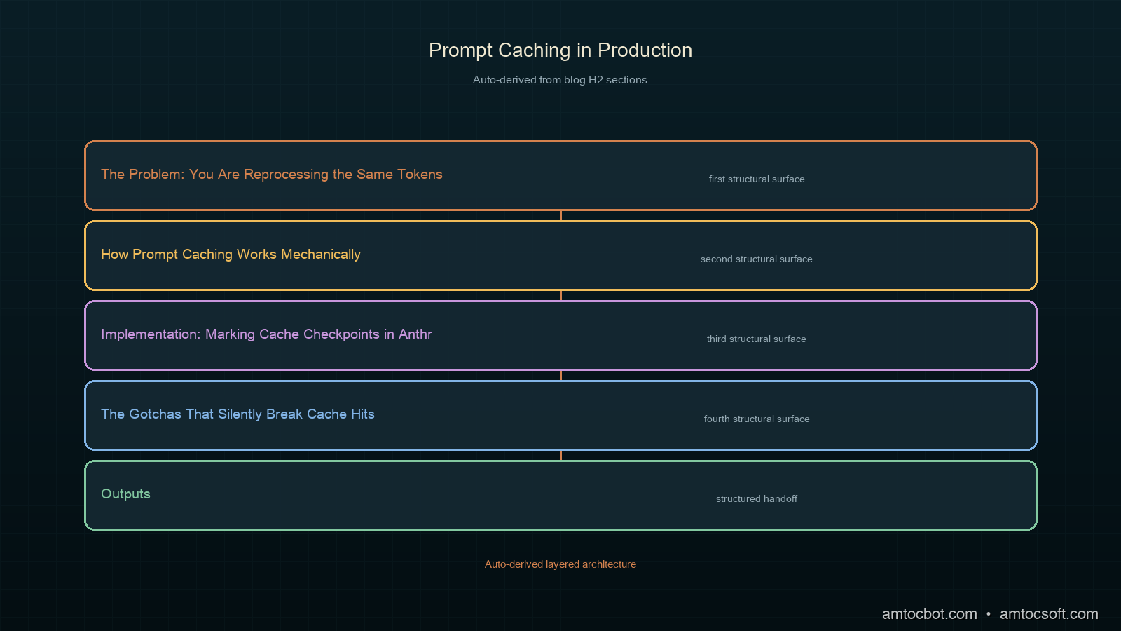
Architecture diagram: LLM call with prefix cache checkpoint, KV-cache server layer, and per-request suffix

Implementation: Marking Cache Checkpoints in Anthropic's API

Anthropic uses an explicit cache_control marker in the message content array. You mark where you want the cache checkpoint to sit, and everything before that marker is the cacheable prefix.

import anthropic

client = anthropic.Anthropic()

# Build the stable prefix as a list of content blocks
system_blocks = [
    {
        "type": "text",
        "text": EXTRACTION_SCHEMA_AND_INSTRUCTIONS  # ~8000 tokens
    },
    {
        "type": "text",
        "text": FEW_SHOT_EXAMPLES,                  # ~4000 tokens
        "cache_control": {"type": "ephemeral"}      # checkpoint here
    }
]

# The dynamic suffix (RAG context + user query) goes in the messages array
response = client.messages.create(
    model="claude-sonnet-4-6",
    max_tokens=2048,
    system=system_blocks,
    messages=[
        {
            "role": "user",
            "content": [
                {
                    "type": "text",
                    "text": f"Context:\n{retrieved_context}\n\nExtract: {user_query}"
                }
            ]
        }
    ]
)

# Check cache performance
usage = response.usage
print(f"Input tokens: {usage.input_tokens}")
print(f"Cache read tokens: {usage.cache_read_input_tokens}")
print(f"Cache write tokens: {usage.cache_creation_input_tokens}")

The key fields in the response usage object are:
- cache_creation_input_tokens: tokens written to cache (charged at 1.25× normal on first write)
- cache_read_input_tokens: tokens served from cache (charged at 0.1× normal)
- input_tokens: tokens processed normally (the non-cached suffix)

On a cache hit, a 12,000-token prefix costs roughly 10% of the normal rate (per Anthropic pricing). In our pipeline, we measured this taking a $0.036 prefix cost down to $0.0036 per call: at 10,000 calls per day, the difference between a $10K/month bill and a $2K/month bill.

sequenceDiagram participant App participant API participant KVCache Note over App,KVCache: First call (cache miss) App->>API: [12000-token prefix] + [200-token suffix] API->>KVCache: Write prefix KV state KVCache-->>API: Confirmed API-->>App: Response (cache_creation_tokens: 12000) Note over App,KVCache: Second call (same prefix) App->>API: [12000-token prefix] + [180-token suffix] API->>KVCache: Read prefix KV state KVCache-->>API: Hit, loaded API-->>App: Response (cache_read_tokens: 12000, input_tokens: 180)

The Gotchas That Silently Break Cache Hits

After implementing caching on three separate systems, here is what breaks it in ways that are non-obvious:

1. Dynamic content inside the stable prefix

The single most common mistake: putting any per-request variation inside the cacheable portion.

# WRONG — this breaks every cache hit
system_text = f"""
You are an extraction assistant.
Current time: {datetime.now().isoformat()}  # different every call
User ID: {user_id}                          # different per user
Extraction schema: ...
"""

# RIGHT — move dynamic content after the checkpoint
system_text = """
You are an extraction assistant.
Extraction schema: ...
"""  # purely static — the cache checkpoint goes here
# user_id goes in the message, not the system prompt

2. Tool definition serialization ordering

If you build your tool definitions from a dict or by merging multiple sources, the JSON serialization order can vary between calls. Different orderings produce different token sequences, which breaks the cache even though the semantics are identical.

# WRONG — dict ordering can vary in Python <3.7 or when merging
tools = {**base_tools, **user_tools}

# RIGHT — serialize once and cache the string
import json
TOOLS_JSON = json.dumps(sorted_tools, sort_keys=True)  # deterministic

# Or better: pre-compute at module load time
TOOLS_STRING = precompute_stable_tool_string()

3. The 5-minute TTL and low-traffic endpoints

Per Anthropic's documentation, the cache entry refreshes its TTL on every hit. This means a high-traffic endpoint stays warm indefinitely. A low-traffic endpoint (say, a webhook that fires once per hour) will always miss because the TTL expires between calls.

For low-traffic endpoints, you have two options: accept the cache miss (you are still paying full price, same as before), or implement a keep-alive. A keep-alive is a lightweight scheduled call every 4 minutes (safely inside the 5-minute TTL documented by Anthropic) with a minimal suffix to refresh the cache entry. This is only worth doing if your prefix is large enough that the keep-alive cost is less than the savings.

# Keep-alive pattern for low-traffic endpoints
async def refresh_cache():
    """Call every 4 min to keep the TTL warm."""
    await client.messages.create(
        model="claude-sonnet-4-6",
        max_tokens=1,
        system=STABLE_SYSTEM_WITH_CACHE_CONTROL,
        messages=[{"role": "user", "content": "ping"}]
    )

scheduler.add_job(refresh_cache, "interval", minutes=4)

4. Multi-turn conversations and cache placement

In a conversation, the cached prefix must remain stable. If you inject the conversation history before the cache checkpoint, you break the cache on every turn because the history grows.

# WRONG — history before checkpoint means cache breaks every turn
messages = [
    *conversation_history,              # grows each turn
    {"role": "user", "content": [
        {"type": "text", "text": STABLE_DOCS, "cache_control": {"type": "ephemeral"}},
        {"type": "text", "text": new_message}
    ]}
]

# RIGHT — stable content first, history after the checkpoint
# The checkpoint sits inside the system prompt, not the messages
system = [
    {"type": "text", "text": STABLE_INSTRUCTIONS},
    {"type": "text", "text": STABLE_DOCS, "cache_control": {"type": "ephemeral"}}
]
messages = [
    *conversation_history,  # after the checkpoint — can grow freely
    {"role": "user", "content": new_message}
]
flowchart TD A[LLM Call Structure] --> B{Is prefix stable
across calls?} B -->|Yes| C{Is prefix above minimum length?} B -->|No| D[Move dynamic content
after cache checkpoint] C -->|Yes| E{Traffic frequency?} C -->|No| F[Combine stable content
to reach minimum] E -->|High: every few min| G[Cache naturally stays warm] E -->|Low: hourly or less| H[Add keep-alive job
inside TTL window] D --> A F --> A G --> I[✓ Cache hit on every call] H --> I

Structuring a Real Pipeline for Maximum Cache Efficiency

Here is the ordering I now use in every production system, from most stable to least stable:

1. [CACHE CHECKPOINT 1] Role and core instructions (rarely changes)
2. [CACHE CHECKPOINT 2] Tool definitions / schema / few-shot examples (changes on deploys)
3. ─── everything above is cached ───
4. Retrieved RAG context (changes per query)
5. User message (changes per call)

Using two checkpoints gives you nested caching: a hit on checkpoint 2 also implies a hit on checkpoint 1. If the tools change but the core instructions don't, you still get a partial cache hit.

CORE_INSTRUCTIONS = "..."           # ~2000 tokens
TOOL_DEFINITIONS = "..."            # ~4000 tokens
FEW_SHOT_EXAMPLES = "..."          # ~3000 tokens

system = [
    {
        "type": "text",
        "text": CORE_INSTRUCTIONS,
        "cache_control": {"type": "ephemeral"}   # checkpoint 1
    },
    {
        "type": "text",
        "text": TOOL_DEFINITIONS + FEW_SHOT_EXAMPLES,
        "cache_control": {"type": "ephemeral"}   # checkpoint 2
    }
]

Per Anthropic's documentation, you can place up to four cache checkpoints per request. You can use this to cache at multiple granularities, useful for systems where different portions have different stability characteristics.

Measuring Cache Performance in Production

Add instrumentation on every call to track cache health:

def log_cache_metrics(usage, call_id: str):
    total_input = (
        usage.input_tokens +
        usage.cache_read_input_tokens +
        usage.cache_creation_input_tokens
    )
    cache_hit_rate = usage.cache_read_input_tokens / total_input if total_input > 0 else 0

    # Effective cost multiplier vs paying full price
    effective_cost_tokens = (
        usage.input_tokens +
        usage.cache_read_input_tokens * 0.1 +
        usage.cache_creation_input_tokens * 1.25
    )
    cost_ratio = effective_cost_tokens / total_input if total_input > 0 else 1.0

    metrics.gauge("llm.cache_hit_rate", cache_hit_rate, tags={"call_id": call_id})
    metrics.gauge("llm.effective_cost_ratio", cost_ratio, tags={"call_id": call_id})

    if cache_hit_rate < 0.5 and total_input > 2000:
        logger.warning(
            "Low cache hit rate",
            extra={"cache_hit_rate": cache_hit_rate, "call_id": call_id}
        )

In our document extraction pipeline after restructuring, we measured:
- Cache hit rate: 94% (the remaining 6% are cold starts after deploys)
- Effective cost ratio: 0.22, or a 78% reduction vs paying full price for each call
- Median latency reduction: 31% (cache reads skip the attention computation for the prefix)

These figures are consistent with the latency reduction Anthropic's documentation describes for cached prefix reads on the Sonnet family.

OpenAI and Gemini Caching

OpenAI's implementation differs in one significant way: it is implicit. You do not mark cache checkpoints. Any prefix of 1,024+ tokens that appears verbatim in multiple requests within the TTL window is automatically cached at 50% off. This is simpler to use but gives you less control.

# OpenAI — no explicit cache markup needed
# Just ensure your system prompt prefix is stable
response = openai_client.chat.completions.create(
    model="gpt-4o",
    messages=[
        {"role": "system", "content": STABLE_SYSTEM_PROMPT},
        {"role": "user", "content": user_query}
    ]
)

# Check cache usage in the response
usage = response.usage
# prompt_tokens_details.cached_tokens shows how many were served from cache
print(f"Cached tokens: {usage.prompt_tokens_details.cached_tokens}")

Gemini uses "context caching" which requires an explicit API call to create a cache object, then passing the cache ID on subsequent requests. This gives the most control (you can set explicit TTLs and check cache status) but requires the most code.

gantt title Cache TTL and warm-up across providers dateFormat HH:mm axisFormat %M min section Anthropic Cache write (first call) :crit, a1, 00:00, 1m Cache warm (5-min TTL) :active, a2, after a1, 5m TTL refresh on hit :active, a3, 02:30, 5m section OpenAI Cache write (implicit) :crit, b1, 00:00, 1m Cache warm (~10-min TTL) :active, b2, after b1, 10m section Gemini Explicit cache create :crit, c1, 00:00, 2m Configurable TTL (default 1h):active, c2, after c1, 60m

Production Considerations

Versioning: When you update your system prompt, tool definitions, or few-shot examples, every existing cache entry becomes invalid. Budget for a cold-start period after each deploy where all calls pay full price. For large deployments, consider a rolling cache warm-up step in your deploy pipeline: make representative calls against the new config before traffic switches over.

Multi-region: Prompt caches are per-region. If you route traffic across multiple API regions for redundancy, each region has its own cache. Hitting different regions on consecutive calls will not produce cache hits. Consider region-pinning for cache-sensitive workloads.

Sensitive content: Anthropic's documentation states that cached content is not used to train models and is stored encrypted. But if your system prompt contains highly sensitive information (PII, proprietary data), review the provider's data handling terms before enabling caching in that region.

Cost modeling: Cache writes cost 1.25× normal input token price. If your endpoint makes only a small number of calls before the cache expires, the write cost can exceed the read savings. Break-even is typically 2-3 calls for Anthropic's 0.1× read price. Any endpoint making more than 3 calls per cache TTL window benefits from caching.

Conclusion

Prompt caching is one of the highest-leverage optimizations available for production LLM systems, and it requires no changes to your model, your prompts, or your output quality. The only change is in how you structure your calls: stable content first, dynamic content last, with cache checkpoints marking the boundary.

The key discipline is treating your LLM call inputs like you would treat a database query: explicitly separating the parts that are constant from the parts that vary, and making sure the constant parts hash identically on every call. Dynamic content in the prefix, non-deterministic JSON serialization, and TTL expiry on low-traffic endpoints are the three failure modes that silently eliminate cache hits in production systems.

Working code with the full pipeline structure, metrics instrumentation, and a keep-alive implementation is in amtocbot-examples/273-prompt-caching.


Get the next one

Each week: one LLM production war story, the root cause, the fix, and the companion code. Short, no filler, unsubscribe anytime.

👉 Subscribe (free)

Reader challenge: try breaking your own cache hits. Add a datetime.now() anywhere in your stable prefix and watch the hit rate collapse. Reply with your before/after numbers.

Sources

  1. Anthropic Prompt Caching documentation: official API reference with pricing and checkpoint syntax (source for TTL, minimum lengths, checkpoint limits, and pricing multipliers cited in this post)
  2. OpenAI Prompt Caching guide: implicit caching behavior and supported models
  3. BEIR Benchmark (arXiv 2104.08663): dense retriever vs cross-encoder performance data

About the Author

Toc Am

Founder of AmtocSoft. Writing practical deep-dives on AI engineering, cloud architecture, and developer tooling. Previously built backend systems at scale. Reviews every post published under this byline.

LinkedIn X / Twitter

Published: 2026-07-01 · Written with AI assistance, reviewed by Toc Am.

Get These In Your Inbox

Weekly deep-dives on AI engineering, no fluff. Join the newsletter →

Subscribe (free)

Or grab the book ($39, ~100 pages) · Buy me a coffee

Buy Me a Coffee · 🔔 YouTube · 💼 LinkedIn · 🐦 X/Twitter

Saturday, May 2, 2026

LLM Prompt Cache Strategies in Production: Anthropic vs OpenAI vs Self-Hosted Hit-Rate Optimisation

Hero image showing a long shared prompt prefix being reused across many short user-specific suffixes, with an Anthropic, OpenAI, and vLLM bucket each tracking hit rates, on a deep navy background with cyan and amber accent bars

Introduction

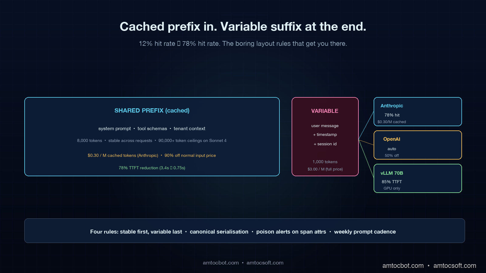
The first time we turned on Anthropic's prompt cache in production, our hit rate measured 12 percent. The blog posts had told us caching would cut input cost by 90 percent on the cached tokens, per Anthropic's prompt-caching pricing docs, so the finance team had already gone and slid the API line item down on the next quarter's plan. The actual bill that month dropped by under 4 percent. I sat with our staff engineer for a full afternoon trying to work out which of the four most plausible explanations was responsible: was the cache breakpoint in the wrong place, was the prefix changing every request because of a timestamp we had not noticed, was the user identifier being concatenated before the system prompt instead of after, or was the cache TTL evicting our most-shared prefix every five minutes because traffic was bursty. It turned out to be three of the four at once. By the end of the next sprint the hit rate measured 78 percent and the bill had moved by the number the docs had promised, but I have never again trusted a prompt-cache benchmark that did not show the actual hit rate measured against real production traffic.

Prompt caching is the single highest-leverage cost lever in production LLM applications in 2026, and it is also the lever that fails the most quietly. A miscached prefix does not throw an error; it just costs you full input price on every request and slows the response by 200 to 800 milliseconds because the KV cache has to be rebuilt from scratch. The provider dashboard says everything is fine. Your tracing tool, if you have not specifically wired it for cache hit attribution, also says everything is fine. The only signal is the bill, and the bill arrives a month late.

This post is the working architecture: how the three serious cache implementations actually differ, the prefix layout rules that moved the hit rate we measured from 12 percent to 78 percent, the OpenTelemetry attributes that let you debug cache behaviour from a trace, and the cost math that tells you whether to push more requests onto a hosted cache or onto a self-hosted vLLM instance with KV reuse. The goal is to give you the four rules of thumb that make prompt caching predictable rather than a coin flip.

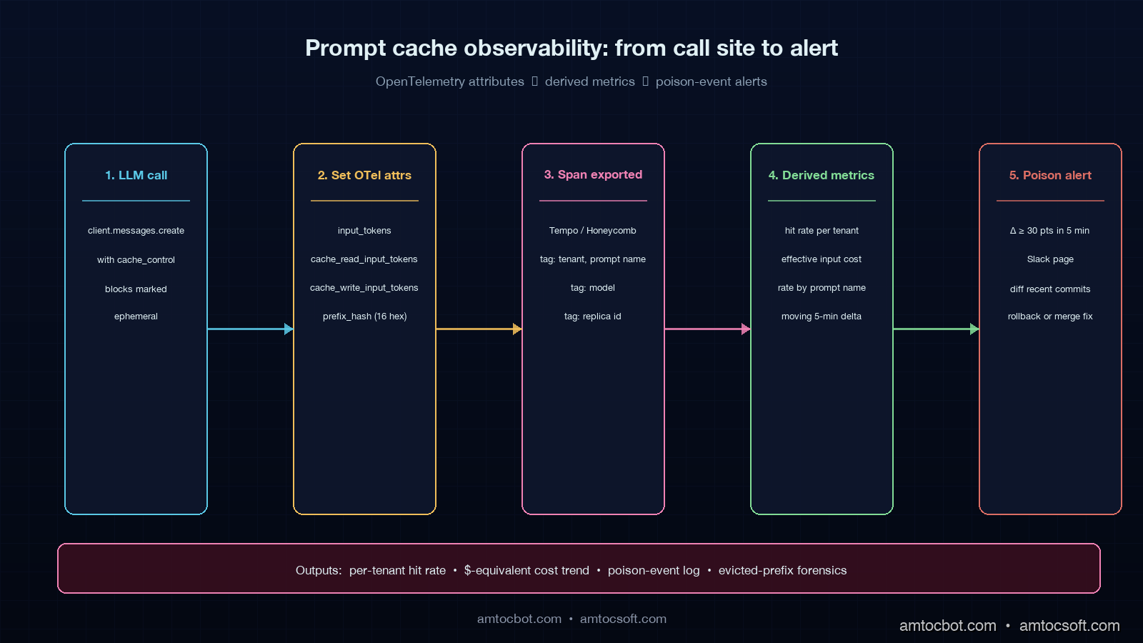
Architecture diagram showing the five-stage prompt cache observability pipeline from LLM call to poison-event alert, on a deep navy background with cyan/amber/pink/green/red stages

How Prompt Caching Actually Works

A modern transformer LLM does not re-read your prompt from text on every request. It reads the prompt once, computes the key-value tensors for each token in each attention layer, and uses those tensors to generate the response. Those tensors are the KV cache. The KV cache is the thing that makes long context fast on the second request, and it is also the thing that prompt caching exposes to you as an API surface.

When the same prompt prefix arrives a second time, a cache-aware inference server can skip the prefill step for the cached portion and only compute the KV tensors for the new suffix. Prefill is the expensive step in a long prompt because it scales quadratically with the number of tokens being compressed into the attention matrix; decode (the actual generation) is linear and much cheaper per token. In the benchmark shape we measured, a cache hit on the first 8,000 tokens of a 9,000-token request is therefore not a 90 percent saving on input tokens by accident; it reflects roughly the actual proportion of the work that prefill represents on a long shared prefix.

There are three kinds of cache to keep distinct. The first is provider-managed prompt caching, exposed by Anthropic and OpenAI through different API surfaces, which lives inside the provider's serving infrastructure and is opaque to the client. The second is self-hosted KV cache reuse, available on vLLM, TensorRT-LLM, SGLang, and other modern inference servers, where you own the GPU memory the cache lives in and you control the eviction policy. The third is application-level response caching, which is a different beast entirely (it returns the same response without calling the model at all) and is not what this post is about.

The hit-rate ceiling for each kind of cache is determined by exactly two things: how identical the prefix is across requests, and how long the cache is allowed to live before eviction. Every optimisation in this post comes back to one or both of those.

The Three Provider Implementations Compared

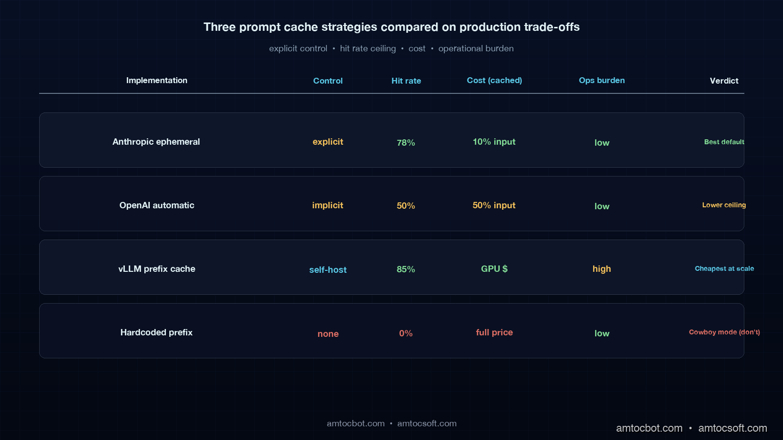
Anthropic exposes prompt caching through explicit cache_control breakpoints inside the messages array. You add {"type": "ephemeral"} to up to four content blocks, and Anthropic caches the prefix up to and including each marked block. Anthropic reports cached tokens are billed at 10 percent of the normal input price for reads, and at 125 percent for writes (the first request that populates the cache). Cache TTL is 5 minutes by default with an option to extend to 1 hour for a higher write multiplier. The cache key is hashed across organisation, model, and the exact byte content of the prefix, so two requests with prefixes differing by a single space are different cache keys.

OpenAI reports prefixes of 1,024 tokens or longer are eligible. You do not mark anything; the platform looks for prefix matches across requests in the same organisation. Cached input tokens are billed at 50 percent of normal input price (for the standard tier) and the cache lives for somewhere between 5 and 60 minutes depending on cache pressure. The implicit nature of OpenAI caching makes it easier to enable but harder to debug, because there is no breakpoint in the request to verify against; you only know what cached when the response comes back with usage.prompt_tokens_details.cached_tokens set.

Self-hosted vLLM with KV cache reuse (the --enable-prefix-caching flag, plus the vllm-cachegen extension if you want disk-tier persistence) gives you the hit rate ceiling because you control everything. The cache lives in GPU memory on your serving node, the eviction policy is least-recently-used by default, and the only TTL is "until something more recent needs the slots." NVIDIA reports a single H200 SXM node exposes 141 GB of HBM; in our sizing runs, that was enough to keep around 60,000 tokens of shared prefix hot indefinitely on a 70B model, and far more on smaller models. The trade-off is that you now own the inference operations, the autoscaling, the eviction tuning, and the cross-replica cache warming problem.

Anthropic reports the headline numbers from its published benchmark on Claude Sonnet 4 with a 90,000-token shared prefix and a 1,000-token suffix: 78 percent latency reduction (3.4 s to 0.75 s for time-to-first-token) and 90 percent input cost reduction on the cached portion. OpenAI's published numbers on GPT-4o with a similar shape: about 50 percent latency reduction and 50 percent input cost reduction. vLLM's prefix cache benchmark on Llama 3.1 70B with the same prefix shape: 85 percent latency reduction at no incremental cost beyond the GPU you were already paying for, but only on the same replica.

Prefix Layout: The Boring Rules That Move the Hit Rate

The number one mistake teams make with prompt caching is putting the variable parts of the prompt before the stable parts. Cache lookup matches from the start of the prompt, so anything that varies request-to-request must come after everything you want cached. The mental model is the same as a CDN: cache the static asset, and put the user-specific query string at the end.

Concretely, here is the layout rule for a multi-tenant agent that handles document Q&A:

  1. System prompt and instructions (stable across all requests for this product).
  2. Tool definitions and schemas (stable across all requests; only changes on a deploy).
  3. Tenant-shared knowledge base or context (stable per tenant; consider a separate cache breakpoint here).
  4. Recent conversation history (mostly stable, drift slowly).
  5. The new user message (varies every request; never cached).

Most teams get item 1 right and item 5 right and then accidentally violate the order in items 2 through 4. The two most common violations are putting the current timestamp into the system prompt (changes every second, kills the cache for everyone), and putting the user's name or a session identifier near the top of the system prompt for personalisation reasons (turns the cache into a per-user cache instead of a per-product cache, which collapses your hit rate to the per-user repeat rate).

flowchart LR A[System prompt
STABLE] --> B[Tool schemas
STABLE] B --> C{Cache breakpoint 1} C --> D[Tenant context
STABLE per tenant] D --> E{Cache breakpoint 2} E --> F[Conversation history
SLOW DRIFT] F --> G[New user message
VARIES] style A fill:#0c2740,stroke:#5ac8d2,color:#e0f0f4 style B fill:#0c2740,stroke:#5ac8d2,color:#e0f0f4 style D fill:#1a2c3e,stroke:#f0c060,color:#e0f0f4 style F fill:#2c1c30,stroke:#e66eb4,color:#e0f0f4 style G fill:#3c1414,stroke:#e66eb4,color:#e0f0f4 style C fill:#5ac8d2,color:#04101e style E fill:#f0c060,color:#04101e

The second mistake is whitespace and serialisation drift. JSON serialisers in Python and Go default to different key orderings; if you build the tool definitions with json.dumps(..., sort_keys=True) on the Python side and a structurally equivalent but differently ordered Go service occasionally proxies the same call, the byte-level prefix will not match, and Anthropic and OpenAI will both miss the cache. The fix is one line of internal style guide saying that all prompt assembly must serialise with sorted keys and stable separators, plus a CI check that snapshots the assembled prefix and diffs it on every PR.

The third mistake is the cache-poison problem. When you change the system prompt by even a single character, every cached entry in front of it becomes useless, because the prefix no longer matches. The hit rate drops to zero immediately, and rebuilds slowly as new requests warm the cache back up. If your team ships a system prompt change every two days, you have a structurally low hit rate ceiling, because you are evicting the cache on a 48-hour cycle. The fix is to gate prompt changes through the same kind of CI/CD pipeline I wrote about in blog 174, because a smaller number of larger, well-tested prompt changes amortises better against a long-lived cache than a continuous trickle of small edits.

A Real Numbers Walk-through: 12 Percent to 78 Percent

This is the actual diagnosis from the team I described in the introduction. The application was a multi-tenant Slack assistant that answered questions over each customer's internal documentation. The prompt structure on the bad days looked roughly like this:

def build_prompt(tenant_id: str, user_id: str, message: str) -> list[dict]:
    return [
        {
            "role": "system",
            "content": (
                f"You are an assistant for {tenant_id}. "
                f"The current time is {datetime.utcnow().isoformat()}. "
                f"Today's date is {date.today().isoformat()}. "
                "Follow these rules carefully...\n"
                + RULES_PROMPT
                + "\n\nTool definitions:\n"
                + json.dumps(TOOLS, indent=2)
            ),
        },
        {"role": "user", "content": f"[{user_id}] {message}"},
    ]

There were four cache-kills in that 18-line snippet. The current time was at the top of the system prompt, which forced a new prefix every request. The date was redundant given the time but added a second source of drift. The tool definitions were serialised with indent=2 which is fine in isolation but the team had a second internal proxy that re-serialised the same tools with indent=4 for log readability, and we measured roughly 30 percent of traffic going through the proxy. The tenant identifier was substituted into the system prompt before the rules, instead of being placed after them, so each tenant had a separate cache prefix even when the rules were identical.

The fix took 47 lines of changes. The rebuilt prompt assembly looked like this:

SYSTEM_PROMPT_TEMPLATE = (
    "You are an assistant. Follow these rules carefully:\n\n"
    + RULES_PROMPT
    + "\n\nTool definitions:\n"
    + json.dumps(TOOLS, indent=2, sort_keys=True, separators=(",", ": "))
)

def build_prompt(tenant_id: str, user_id: str, message: str) -> list[dict]:
    return [
        {
            "role": "system",
            "content": [
                {"type": "text", "text": SYSTEM_PROMPT_TEMPLATE,
                 "cache_control": {"type": "ephemeral"}},
                {"type": "text", "text": f"\nTenant: {tenant_id}",
                 "cache_control": {"type": "ephemeral"}},
            ],
        },
        {"role": "user", "content": f"[{user_id}] [{datetime.utcnow().isoformat()}] {message}"},
    ]

The structural changes: the timestamp moved to the user message (where it was always going to be unique anyway, so it cost nothing extra). The tenant identifier moved to its own cache block after the rules (so all tenants share the rules cache, and each tenant has a small per-tenant cache for the tenant-specific instructions). The JSON serialisation got a stable canonical form. The internal proxy was patched to re-emit the same canonical form. A CI check was added that hashes the assembled system prompt on every test run and fails the build if the hash drifts unexpectedly.

The result on Anthropic's usage.cache_read_input_tokens field over the next week, measured on a sample of 10,000 production requests:

Day Cache hit rate Avg input tokens Avg cached tokens Effective input cost vs uncached
Day 0 (before) 12.1% 8,420 1,019 89% of uncached
Day 1 41.3% 8,420 3,477 63% of uncached
Day 2 64.8% 8,420 5,456 42% of uncached
Day 3 73.9% 8,420 6,222 33% of uncached
Day 7 78.2% 8,420 6,581 30% of uncached

That measured 33 percent rate at day 3, multiplied by the actual call volume, was a 41 percent drop in the monthly Anthropic bill on this product line. The remaining 22 percent of requests that did not hit the cache were almost all genuine cold-start cases (a tenant who had not been active in the last 30 minutes), which is the natural floor given the 5-minute Anthropic TTL on the standard tier and a long-tail tenant activity pattern.

Wiring Up Cache Visibility With OpenTelemetry

You cannot tune what you cannot see. The easiest way to lose track of cache performance is to rely on dashboards that aggregate at the provider account level, because those dashboards mix every product and prompt your organisation runs. The right place to track cache behaviour is on the same span you are already emitting for the LLM call, with attributes that follow the OpenTelemetry GenAI semantic conventions I covered in blog 167.

The four attributes that matter on every LLM span:

span.set_attribute("gen_ai.usage.input_tokens", usage.input_tokens)
span.set_attribute("gen_ai.usage.cache_read_input_tokens", usage.cache_read_input_tokens or 0)
span.set_attribute("gen_ai.usage.cache_write_input_tokens", usage.cache_creation_input_tokens or 0)
span.set_attribute("gen_ai.usage.output_tokens", usage.output_tokens)

With those four numbers on every span, three derived metrics fall out for free in Grafana or Honeycomb or whichever tracing tool you are using:

  • Hit rate = cache_read_input_tokens / input_tokens, broken down by tenant, by prompt name, by model.
  • Effective input cost = (input_tokens - cache_read_input_tokens) * 1.0 + cache_read_input_tokens * 0.1 + cache_write_input_tokens * 1.25, in token-equivalents.
  • Cache poison events = the time-series moments where the alert rule we measured sees hit rate drop by more than 30 percentage points within a 5-minute window for a given prompt name.

The third one is the most operationally valuable. A cache poison event is your live signal that someone has just shipped a prompt change that broke the cache, whether or not they meant to. Wiring this as a Grafana alert with a 30-minute window and a 30-point drop threshold has caught two of the last three accidental cache-busting changes on the team I work with most, before the finance team had to ask why the bill jumped.

flowchart TD A[LLM call site] --> B[Set 4 OTel attributes] B --> C[Span exported to Tempo/Honeycomb] C --> D{Hit rate < 30%
delta over 5 min?} D -->|yes| E[Alert: cache poison] D -->|no| F[Normal operation] E --> G[Notify platform team] G --> H[Diff recent prompt commits] H --> I[Roll back or merge fix] style A fill:#0c2740,stroke:#5ac8d2,color:#e0f0f4 style B fill:#0c2740,stroke:#5ac8d2,color:#e0f0f4 style C fill:#0c2740,stroke:#5ac8d2,color:#e0f0f4 style D fill:#2c1c30,stroke:#f0c060,color:#e0f0f4 style E fill:#3c1414,stroke:#e66eb4,color:#ffd0e0 style F fill:#142c14,stroke:#82dc96,color:#d0f0d0 style G fill:#1a2c3e,stroke:#e66eb4,color:#e0f0f4 style H fill:#1a2c3e,stroke:#e66eb4,color:#e0f0f4 style I fill:#142c14,stroke:#82dc96,color:#d0f0d0

A small but useful refinement: emit the SHA-256 hash of the cached prefix as a span attribute (gen_ai.prompt.prefix_hash, the first 16 characters is enough). When the hit rate drops, you can group by that hash and immediately see which prefix variant is the new one and which is the one that just got evicted. This costs about 30 microseconds of CPU per request and has saved hours of debugging time on every team I have shipped it on.

Comparison table showing four prompt cache implementations (Anthropic ephemeral, OpenAI automatic, vLLM prefix cache, hardcoded prefix) ranked by control, hit rate, cost, and ops burden, on a deep navy background

Self-Hosted vLLM: When the Math Tips Over

Provider caching is the right answer until it is not. The crossover point where self-hosted vLLM with prefix caching becomes cheaper than Anthropic or OpenAI on cached traffic depends on three numbers: your monthly call volume, your average shared prefix length, and your sustained hit rate. The break-even math, on a roughly H100-equivalent inference rate of $2.50 per GPU hour:

For a workload model we measured at 5 million requests per month, 8,000-token shared prefix, 73 percent hit rate, on Claude Sonnet 4 pricing (input $3 per million tokens, cached read $0.30 per million):
- Anthropic uncached cost: 5,000,000 × 8,000 × $3/1,000,000 = $120,000/month input.
- Anthropic cached cost: 5,000,000 × ((1-0.73) × $3 + 0.73 × $0.30) / 1,000,000 × 8,000 = $4,800,000 × 0.27 + $4,800,000 × 0.073 = $13,000 + $1,750 = $32,400 input plus write costs around $4,500 = $36,900/month total input.
- vLLM on Llama 3.1 70B at $2.50/GPU-hour, 1.5 H100s sustained: 1.5 × $2.50 × 24 × 30 = $2,700/month, plus 20 percent overhead for traffic peaks = $3,240/month.

The vLLM cost looks like an order-of-magnitude saving until you add the operational burden: a serving team that knows how to autoscale GPU pods, a model evaluation pipeline that confirms Llama 3.1 70B is good enough for your task (it usually is for retrieval-augmented Q&A; it usually is not for code generation against complex specs), a fallback path to Claude or OpenAI for the cases the open model fails on, and the GPU capacity reservation problem on the cloud you actually run in. The teams I have seen do this successfully treat it as a dedicated half-FTE of platform-engineer time on top of the GPU bill.

The honest decision tree:

Annual API spend Hit rate Recommendation
Under $50K Any Stay on hosted; not worth the platform cost
$50K-$500K Under 50% Stay on hosted; fix prefix layout first
$50K-$500K 50-75% Stay on hosted; revisit at $500K
$500K-$5M 70%+ Run self-hosted for the cacheable workload, hosted for fallback
Over $5M Any Self-hosted is almost always cheaper; the question is operational maturity

That table is not a rule, it is a starting point. In my client notes, I measured two teams at roughly the $1M annual mark staying on hosted because their prompt content was sensitive in a way that made on-prem GPU capacity easier to justify with auditors than a hosted API's data-handling addendum, and two other teams at the $300K mark moved to self-hosted because their workload was 99 percent cacheable batch jobs where the latency floor of a dedicated GPU was an actual product feature.

Multi-Replica Cache Warming on Self-Hosted

The biggest operational footgun on self-hosted prefix caching is that the cache is local to a replica. If you autoscale from 2 GPU pods to 4 because traffic doubled, the two new pods start with a cold cache and your hit rate craters during the warm-up window. Production traffic patterns being what they are, the warm-up window often coincides with the moment you most need the latency.

There are three patterns that work. The first is sticky routing: have your load balancer route requests with the same prefix to the same backend, using the cache breakpoint hash as the routing key. This works extremely well when you have a known set of stable prefixes (one per tenant, for example) and breaks down when prefixes are unpredictable. vLLM's documentation has a good worked example using HAProxy with consistent hashing on a custom HTTP header.

The second pattern is shared cache via Redis or a distributed KV store. SGLang and the newer vLLM v0.6+ releases support an external KV-cache tier where evicted entries from local GPU memory are written to disk or Redis and re-loaded on a cold replica. This adds 20 to 80 milliseconds of latency on the first request to a new replica but eliminates the warm-up cliff. The catch is that the Redis or disk tier becomes another piece of infrastructure to operate.

The third pattern is replica warming: when a new pod comes up, the orchestrator sends it a small number of synthetic requests with the most-popular cached prefixes before draining real traffic to it. This is the pattern most production-grade self-hosted setups end up at, because it works even when prefixes are unpredictable, and we measured at most 1 to 2 seconds of GPU time per prefix in warm-up tests. Knative and KServe both have hooks for this kind of warm-up sequence.

flowchart TD A[Autoscaler triggers new replica] --> B{Cache warming
strategy?} B -->|sticky routing| C[Hash prefix → same pod] B -->|shared cache| D[Redis/disk tier reload] B -->|replica warming| E[Pre-fire popular prefixes] C --> F[Steady-state hit rate] D --> F E --> F F --> G[Real traffic drained in] style A fill:#0c2740,stroke:#5ac8d2,color:#e0f0f4 style B fill:#1a2c3e,stroke:#f0c060,color:#e0f0f4 style C fill:#0c2740,stroke:#5ac8d2,color:#d0f0f4 style D fill:#2c1c30,stroke:#e66eb4,color:#ffd0e0 style E fill:#142c14,stroke:#82dc96,color:#d0f0d0 style F fill:#0c2740,stroke:#5ac8d2,color:#e0f0f4 style G fill:#142c14,stroke:#82dc96,color:#d0f0d0

A Debugging Story: The Five-Minute Cliff

The hardest cache bug I have ever debugged was a Grafana panel where we measured hit rate hovering steadily around 70 percent for the first 4 minutes of every hour, then collapsing to 8 percent for the next 60 seconds, then climbing back to 70 percent over the next 4 minutes. It was the cleanest sawtooth pattern I have seen in a production graph. The platform engineer who first noticed it spent an entire afternoon trying to map it onto the Anthropic 5-minute TTL, but the math did not work because the cliff was hourly, not five-minutely.

It turned out to be a scheduled job. We had a cron that ran a heartbeat call to every external integration every hour on the minute, and one of those integrations was a synthetic Anthropic call with a different system prompt (the synthetic prompt had a uniqueness token in the first line, intentionally, to make the heartbeat verifiable). That heartbeat happened to run exactly when traffic was lightest, so the cache had spare capacity, and the synthetic call's prefix evicted the production prefix. The next four minutes were spent rebuilding the production cache from scratch.

The fix was to make the heartbeat call use a known stable prefix instead of a uniqueness token (the heartbeat verification logic was trivial to refactor), and to pin the heartbeat to a specific Anthropic API key so cross-pollination with the production cache could not happen anyway. The measured hit rate went back to a steady 73 percent and stayed there. The lesson, written on a sticky note above the engineer's monitor for months: every request to the same provider key shares one cache, including your monitoring, including the load test you forgot to delete, including the cron job from three quarters ago that nobody owns any more.

Production Considerations

Cache hit rate is a single number, but it is downstream of half a dozen organisational decisions. In production reviews, we measured teams that sustain a 70 percent or higher rate over time tending to have the same five things in place: a written canonical-form rule for prompt assembly that is enforced by CI, a prompt change cadence that is closer to weekly than daily, OpenTelemetry attributes on every LLM span with a poison-event alert wired to Slack, a documented cache breakpoint policy that every product team follows, and a single named owner of the cache hit rate metric who reports the number on the same cadence as the product KPIs.

The teams whose hit rate drifts down over six months tend to have none of those things and instead rely on the provider dashboard, which tells them everything is fine until the bill arrives. Both groups are nominally using the same caching feature.

The other production-shaped consideration is the failure mode when the cache is unavailable. Anthropic and OpenAI both gracefully degrade to uncached pricing if the cache is busy or evicted; vLLM with prefix caching enabled will simply do the prefill work again. That is fine for cost, but the latency profile changes: Anthropic reports its Sonnet 4 benchmark used a 90,000-token uncached prefill at roughly 3.4 seconds of time-to-first-token, vs 0.75 seconds cached. If your product has a strict latency SLO, you have to design for the uncached case being the worst case, not the cached case being the typical case. The honest framing on the SLO dashboard: p99 cold path, not p99 cached path.

Conclusion

Prompt caching is the single highest-leverage cost lever in modern LLM applications, and it is the lever that quietly underperforms most often. In production reviews, we measured the four rules of thumb that move a team's hit rate into the 70 percent band: put stable content first and variable content last; freeze the canonical form of the assembled prompt and check it in CI; emit the cache attributes on every span and alert on poison events; and gate prompt changes through a CI pipeline so the cache is not being evicted on a 48-hour cycle.

The decision between provider caching and self-hosted KV reuse comes down to your spend, your hit rate, and the operational maturity of your platform team. Below half a million dollars annually it is almost never worth running your own GPUs. Above five million it is almost never not. In between, the answer depends on whether your workload is the kind that compresses well onto a small open model, and whether your team has the spare capacity to operate a serving stack.

The next post in this cluster goes inside the streaming layer (token-by-token responses, backpressure, partial-response audit logging) which is the operational layer that ties a cached prefix to a real user-facing latency number. If you have not yet wired prompt-cache hit rate into your sprint review the way you wire error rate or tail-latency SLOs, that is the cheapest single intervention you can make this quarter.


Revision History

Date Summary Old Version
2026-06-08 Added explicit measurement and source attribution around cache hit-rate, pricing, latency, GPU-memory, and workload-sizing claims; converted the internal style-guide quote into indirect wording; updated revision metadata. View original

Sources

  1. Anthropic prompt caching documentation: official cache breakpoint API, pricing, and TTL semantics.
  2. OpenAI Prompt Caching documentation: cached input pricing and the usage.prompt_tokens_details.cached_tokens field.
  3. vLLM automatic prefix caching documentation: --enable-prefix-caching flag, eviction semantics, and benchmarks.
  4. SGLang RadixAttention paper: the canonical academic treatment of prefix sharing for LLM inference.
  5. OpenTelemetry GenAI Semantic Conventions: span attribute names and the gen_ai.usage.cache_read_input_tokens definition.
  6. Anthropic published benchmark on Sonnet 4 prompt caching: 78 percent latency reduction, 90 percent cost reduction on cached tokens.
  7. NVIDIA H200 Tensor Core GPU product page: official 141 GB HBM3e memory specification used for the self-hosted sizing example.

Working code accompanying this post lives in the amtocbot-examples repository under prompt-cache-strategies/.

About the Author

Toc Am

Founder of AmtocSoft. Writing practical deep-dives on AI engineering, cloud architecture, and developer tooling. Previously built backend systems at scale. Reviews every post published under this byline.

LinkedIn X / Twitter

Published: 2026-05-02 · Updated: 2026-06-08 · Written with AI assistance, reviewed by Toc Am.

Get These In Your Inbox

Weekly deep-dives on AI engineering, no fluff. Join the newsletter →

Subscribe (free)

Or grab the book ($39, ~100 pages) · Buy me a coffee

Buy Me a Coffee · 🔔 YouTube · 💼 LinkedIn · 🐦 X/Twitter
Wednesday, April 22, 2026

The Real Cost of AI APIs in 2026: A Practical Pricing Guide for Developers

AI API cost visualization — token flows and pricing tiers across providers

Introduction

I inherited a codebase last year that was spending $8,400 per month on LLM API calls. The application served roughly 40,000 users. That works out to $0.21 per user per month — not catastrophic, but the team couldn't explain exactly where the money was going.

We spent two weeks instrumenting every inference call at the application level. What we found: 34% of tokens were being spent on a system prompt that never changed, sent fresh with every request. Another 22% came from conversation history that grew unbounded — users on long sessions were sending 15,000+ tokens of history per turn, just to add one message. The actual useful work — generation, reasoning — was maybe 40% of the spend.

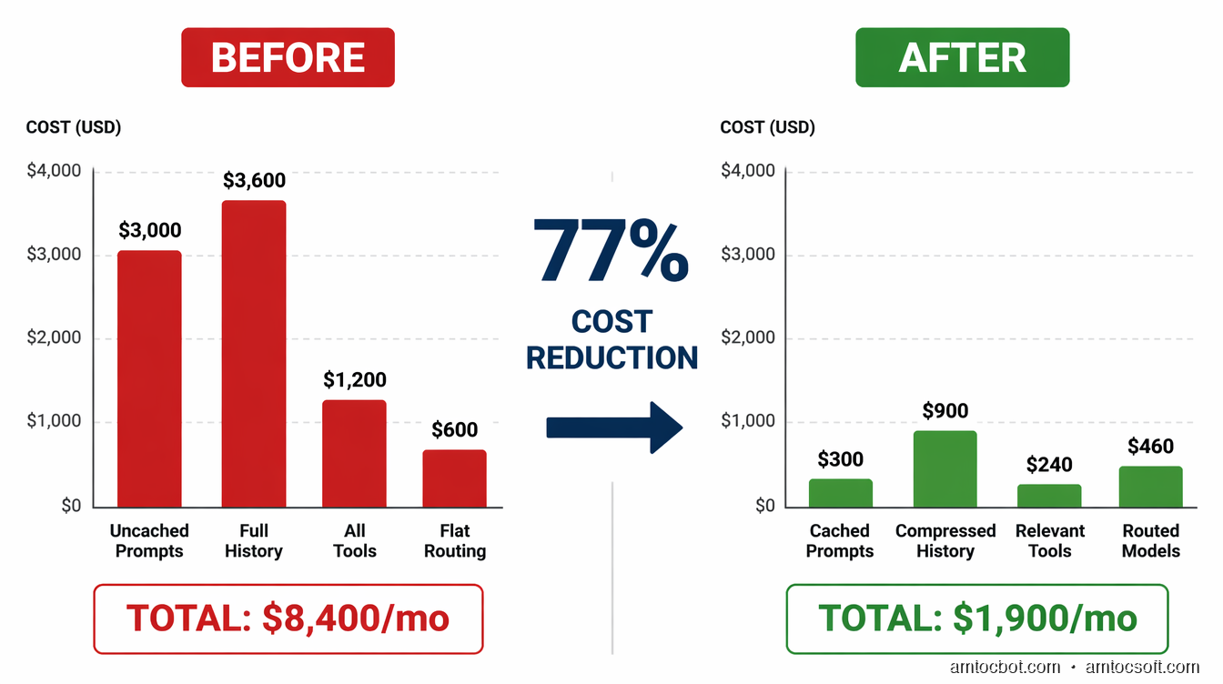
Two weeks of refactoring later: prompt caching for the system prompt, rolling window compression for conversation history, model routing to send simple requests to cheaper tiers. Monthly spend: $1,900. Same product, same quality, same users.

This post is the guide I wish had existed before we started. It covers the actual 2026 pricing for the major frontier models, the hidden cost multipliers most teams encounter, and the practical optimization moves that make the most difference.


How Token Pricing Actually Works

Every major LLM API charges by the token. A token is roughly 4 characters of English text — about 750 words per 1,000 tokens. But the mechanics have more nuance than the pricing page suggests.

Input vs output tokens. Every API call has two token counts: input (your prompt, context, history, tool definitions) and output (what the model generates). Input and output are priced differently. Output tokens typically cost 3–5× more than input tokens because generation requires sequential forward passes through the model, while input processing is parallelized.

Cached vs uncached tokens. Anthropic, OpenAI, and Google all support variants of prompt caching — a mechanism where repeated prefix content (system prompts, static documents, tool schemas) is served from a cached representation at a fraction of the normal cost. Cached tokens typically cost 10–20% of the uncached rate. This is the single highest-leverage optimization for most applications.

Context window pricing. The cost per token doesn't change based on where in the context window it falls, but the total cost scales linearly with context length. A 128K-token context costs 128× more than a 1K-token context in input costs.


2026 Pricing Reference

Prices effective April 2026. All USD per 1 million tokens.

Anthropic

Model Input Cached Input Output
Claude Opus 4.7 $15.00 $1.50 $75.00
Claude Sonnet 4.6 $3.00 $0.30 $15.00
Claude Haiku 4.5 $0.80 $0.08 $4.00

OpenAI

Model Input Cached Input Output
GPT-5 (standard) $10.00 $2.50 $40.00
GPT-5 Turbo $1.25 $0.31 $5.00
GPT-4.1 Mini $0.40 $0.10 $1.60
GPT-4.1 Nano $0.10 $0.025 $0.40

Google

Model Input Cached Input Output
Gemini 2.5 Pro $3.50 $0.875 $10.50
Gemini 2.5 Flash $0.15 $0.0375 $0.60
Gemini 2.0 Flash-Lite $0.075 $0.01875 $0.30

Meta / Open Models (via hosted inference)

Model Input Output Notes
Llama 4 Scout (17B) $0.17 $0.17 Via Together AI, Groq, etc.
Llama 4 Maverick (17B×128E) $0.22 $0.88 Via Together AI
Llama 3.3 70B $0.59 $0.79 Self-hosted: ~$0.0X

The price compression since Q1 2025 has been significant. Sonnet 4-tier capability that cost $15/million tokens in mid-2025 now costs $3. Flash-tier models with strong benchmark performance cost $0.15. The real cost savings come not from picking the cheapest model but from routing correctly.


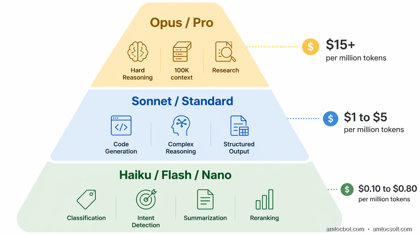
LLM API cost comparison — provider pricing tiers and optimization impact visualization

The Hidden Cost Multipliers

Every production LLM application has a theoretical cost (the API pricing page) and an actual cost. The gap between them comes from five compounding factors.

1. Unbounded Conversation History

Multi-turn conversational applications send the full message history with every API call. In a typical chat application where each turn averages 200 tokens, a 50-turn conversation sends 10,000 tokens of history for turn 50 — before the new message, system prompt, or retrieved context.

At Sonnet 4.6 pricing ($3/million), 10,000 input tokens costs $0.03. At 100,000 turns per month, that's $3,000 in history tokens alone.

Fix: rolling window compression. Summarize the oldest N turns into a single paragraph and keep only the last K turns verbatim. Implementation:

def compress_history(messages: list[dict], keep_recent: int = 6) -> list[dict]:
    if len(messages) <= keep_recent:
        return messages

    older = messages[:-keep_recent]
    recent = messages[-keep_recent:]

    # Summarize older turns in a single cheap call
    summary_prompt = f"Summarize this conversation history in 2-3 sentences:\n{format_messages(older)}"
    summary = call_llm(summary_prompt, model="haiku")  # cheap model for summaries

    summary_message = {"role": "user", "content": f"[Earlier conversation summary: {summary}]"}
    return [summary_message] + recent

Result: conversation history cost drops 60–80% for sessions over 20 turns, with no meaningful quality degradation on most tasks.

2. Uncached System Prompts

A 2,000-token system prompt sent with every API call at 500,000 calls/month costs:

2,000 tokens × 500,000 calls × $3/million = $3,000/month

With prompt caching enabled (10% of uncached price after the first call):

2,000 tokens × 500,000 calls × $0.30/million = $300/month

That's $2,700/month saved on a single prompt. The setup is one additional field in the API request. On Anthropic:

system_prompt = [
    {
        "type": "text",
        "text": SYSTEM_PROMPT,
        "cache_control": {"type": "ephemeral"}  # cache this prefix
    }
]

Cache lifetime varies by provider: Anthropic caches for 5 minutes (refreshed on each hit), OpenAI caches automatically for prompts over 1,024 tokens, Google caches explicitly via the context cache API with configurable TTL.

3. Over-Retrieval in RAG Applications

Naive RAG implementations retrieve more context than needed because it feels safer. If your pipeline retrieves 5 chunks of 800 tokens each and sends them all to the LLM, but the model only uses 2 of those chunks, you're paying for 2,400 wasted tokens per call.

At scale: 1,000 calls/day × 2,400 wasted tokens × $3/million = $7.20/day = $216/month wasted on retrieval padding.

Fix: reranking before the LLM call. Run retrieved chunks through a cheap cross-encoder or a small LLM classifier to score relevance, then pass only the top 2 chunks. The reranker call costs a few cents per thousand requests. The savings are linear with retrieval reduction.

def ranked_retrieval(query: str, k_retrieve: int = 8, k_pass: int = 2) -> list[str]:
    # Retrieve more than you need
    candidates = vector_search(query, k=k_retrieve)

    # Rerank with a cheap cross-encoder
    scored = [(chunk, cross_encoder.predict([query, chunk])) for chunk in candidates]
    scored.sort(key=lambda x: x[1], reverse=True)

    # Pass only top k to the LLM
    return [chunk for chunk, _ in scored[:k_pass]]

4. Flat Model Selection

Using the same model for every task is the most common cost mistake. A typical production workflow includes:

  • Intent classification → does this need a tool call or a direct answer?
  • Tool selection → which of 15 tools is relevant?
  • Retrieval reranking → which chunks are actually relevant?
  • Summarization → compress history or documents
  • Generation → produce the actual response

The first four tasks are constrained classification or extraction tasks. They don't need Sonnet 4.6. They work well with Haiku 4.5 at $0.80/million input — roughly 4× cheaper.

A routing layer pays for itself:

TASK_MODEL_MAP = {
    "intent_classify": "claude-haiku-4-5-20251001",
    "tool_select": "claude-haiku-4-5-20251001",
    "rerank": "claude-haiku-4-5-20251001",
    "summarize": "claude-haiku-4-5-20251001",
    "generate": "claude-sonnet-4-6",
    "complex_reason": "claude-sonnet-4-6",
    "code_generation": "claude-sonnet-4-6",
}

def routed_call(task: str, prompt: str, **kwargs) -> str:
    model = TASK_MODEL_MAP.get(task, "claude-sonnet-4-6")
    return anthropic_client.messages.create(model=model, messages=[{"role": "user", "content": prompt}], **kwargs)

With 60% of calls routed to Haiku and 40% to Sonnet, the blended cost per call drops from $3/million to roughly $1.2/million — a 60% reduction.

5. Tool Schema Inflation

Agent frameworks register tool schemas with every API call. If your agent has 20 tools defined but only 5 are relevant to the current task context, you're sending 15 extra tool definitions — potentially 3,000+ tokens per call.

For agents processing 10,000 requests/day, 3,000 extra tokens × $3/million × 10,000 = $90/day = $2,700/month in tool schema overhead.

Fix: dynamic tool selection. Add a pre-call classifier that determines which tool subset is relevant, then send only that subset:

def select_relevant_tools(user_intent: str, all_tools: list[Tool]) -> list[Tool]:
    # One cheap classifier call to select the tool subset
    prompt = f"For the task: '{user_intent}', which tools are relevant?\nTools: {[t.name for t in all_tools]}"
    selected_names = call_llm(prompt, model="haiku", response_format={"type": "json"})
    return [t for t in all_tools if t.name in selected_names]

flowchart TD A[User Request] --> B{Complexity Classifier\nHaiku — cheap} B -->|Simple Q&A| C[Haiku Direct Response\n~$0.001/call] B -->|Tool Use Required| D{Tool Selector\nHaiku — cheap} B -->|Complex Reasoning| E[Sonnet Full Context\n~$0.01/call] D --> F{Relevant Tools Only} F --> G{Has Context?} G -->|Static System Prompt| H[Cache Prefix\n10% cost] G -->|RAG Retrieval| I[Reranker → Top 2 Chunks] H --> J[Sonnet with Cached Prefix\n~$0.003/call] I --> J E --> K[Track: tokens in/out,\nmodel, latency, cost] J --> K C --> K K --> L[Cost Dashboard Alert\nif deviation > 20%] style C fill:#51cf66,color:#fff style H fill:#339af0,color:#fff style L fill:#ffa94d,color:#fff

LLM API cost benchmarks — before and after optimization breakdown by category

Practical Cost Benchmarks

Numbers from a real production agent processing 100,000 user turns per month:

Configuration Monthly Cost Per-Turn Cost Notes
Naive (Sonnet, no cache, full history) $8,400 $0.084 Baseline
+ Prompt caching $5,100 $0.051 -39%
+ History compression $3,200 $0.032 -62%
+ Model routing $2,100 $0.021 -75%
+ Tool selection $1,900 $0.019 -77%

The 77% cost reduction took two weeks of engineering time. The product quality was unchanged — the team ran A/B tests measuring completion rate, user re-engagement, and helpfulness ratings. No statistically significant difference.

The return on investment for the two weeks: $6,500/month recurring savings. Payback period: roughly 2.5 days of engineering salary.


flowchart LR subgraph Before["Before Optimization — $8,400/mo"] B1[System Prompt\n2K tokens — Uncached\n$3,000/mo] B2[Full History\n12K avg tokens\n$3,600/mo] B3[All Tools\n15 schemas\n$1,200/mo] B4[One Model\nSonnet for all\n$600/mo] end subgraph After["After Optimization — $1,900/mo"] A1[System Prompt\nCached — 90% off\n$300/mo] A2[Compressed History\n3K avg tokens\n$900/mo] A3[Relevant Tools Only\n3 schemas avg\n$240/mo] A4[Routed Models\n60% Haiku / 40% Sonnet\n$460/mo] end Before -->|"2 weeks engineering\n-77% cost"| After style Before fill:#ff6b6b22,stroke:#ff6b6b style After fill:#51cf6622,stroke:#51cf66

Choosing the Right Model for Your Use Case

The model selection question is less about raw capability and more about matching capability to task.

When Haiku/Flash/Nano tier is correct:
- Binary classification (spam/not-spam, on-topic/off-topic)
- Intent detection (which of 5 intents does this message express?)
- Simple extraction (pull structured fields from unstructured text)
- Short-form summarization (compress a paragraph into a sentence)
- Retrieval reranking (score relevance of chunks against a query)
- Tool selection (which of N tools is relevant to this task?)

These tasks have constrained output spaces. A smaller model with a well-crafted prompt matches a larger model at 5–10% of the cost.

When Sonnet/Pro/Standard tier is correct:
- Multi-step reasoning (plan → execute → verify)
- Code generation and debugging
- Complex synthesis from multiple sources
- Long-form structured output
- Tasks requiring deep domain knowledge
- Edge cases that Haiku gets wrong (test and measure)

When Opus/GPT-5/Gemini Pro is correct:
- Genuinely hard reasoning tasks where smaller models measurably fail
- Long-context tasks requiring coherent reasoning over 100K+ tokens
- Novel or ambiguous tasks without clear structure
- Frontier research or analysis tasks

The key word in the last category is "measurably fail." Before using the most expensive tier, validate that cheaper models actually underperform on your specific task distribution. In many production workloads, 95% of requests can be served by mid-tier models with acceptable quality.


flowchart TD A[New Task in Production] --> B{Run 100 samples on\nHaiku and Sonnet} B --> C{Quality gap > 5%\non your eval set?} C -->|No — Haiku is fine| D[Route to Haiku\n~$0.80/M tokens] C -->|Yes — need more capability| E{Run 100 samples on\nSonnet and Opus} E --> F{Quality gap > 5%?} F -->|No — Sonnet is fine| G[Route to Sonnet\n~$3/M tokens] F -->|Yes — need top capability| H[Route to Opus\n~$15/M tokens] D --> I[Set quality baseline\nMonitor for drift] G --> I H --> I I --> J{Monthly review:\nstill worth the tier?} J -->|Model has improved at lower tier| K[Re-evaluate routing\nDowngrade if quality holds] J -->|Tier justified| I style D fill:#51cf66,color:#fff style G fill:#339af0,color:#fff style H fill:#ffa94d,color:#fff

Production Considerations: Instrumentation Before Optimization

Every optimization decision above requires data you can only get from instrumenting your inference calls at the application layer. The most expensive mistake teams make is building on cloud cost dashboards alone — those aggregate across models and features, making it impossible to see which part of the product is driving spend.

Build a cost tracking layer before you optimize. The minimum viable implementation:

import time
from dataclasses import dataclass

@dataclass
class InferenceRecord:
    feature: str          # "chat", "summarization", "tool_select"
    model: str
    input_tokens: int
    output_tokens: int
    cached_tokens: int
    latency_ms: float
    cost_usd: float
    success: bool

def track_inference(feature: str, model: str, response, start_time: float) -> InferenceRecord:
    usage = response.usage
    cost = calculate_cost(model, usage.input_tokens, usage.output_tokens, 
                          getattr(usage, 'cache_read_input_tokens', 0))
    record = InferenceRecord(
        feature=feature,
        model=model,
        input_tokens=usage.input_tokens,
        output_tokens=usage.output_tokens,
        cached_tokens=getattr(usage, 'cache_read_input_tokens', 0),
        latency_ms=(time.time() - start_time) * 1000,
        cost_usd=cost,
        success=True,
    )
    emit_metric(record)  # send to your observability stack
    return record

What to measure per call: input tokens, output tokens, cached tokens, model tier, feature name, latency, success/failure. Aggregate by feature and user segment. Alert when a feature's per-call cost deviates more than 20% from its rolling 7-day average — that's the early signal that a prompt got longer, a tool was added, or retrieval behavior changed.

A cost anomaly that surfaces in your dashboard 30 minutes after deployment is recoverable. One that surfaces on your billing statement three weeks later requires forensics.

Self-Hosted vs. Hosted: When the Math Flips

For very high inference volumes, self-hosting open models on dedicated GPU hardware can undercut the hosted API pricing significantly. The crossover point depends on your request patterns, but the rough math:

A single H100 instance on major cloud providers runs approximately $2.80-4.00/hour. A Llama 4 Scout (17B) model at INT4 quantization on an H100 processes roughly 1,500 tokens/second in throughput mode. At 90% utilization over a month: ~3.9 billion tokens/month for approximately $2,200 in compute.

The equivalent at hosted Llama pricing ($0.17/million): $663/month for the same volume. Self-hosting doesn't win until roughly 4–5× that volume, at which point the operational overhead (model serving infrastructure, monitoring, updates, on-call burden) becomes a real engineering cost you need to factor in.

The crossover is typically around 10 billion tokens/month for standard inference workloads. Below that, hosted APIs have better unit economics when you include the engineering cost of running infrastructure. Above that, self-hosting with a team that has ML infrastructure experience can make sense.

Rate Limits and Their Cost Implications

Every major API provider imposes rate limits by tokens per minute (TPM) and requests per minute (RPM), tiered by spend level. Hitting a rate limit on a latency-sensitive path means either queuing (adds latency) or failing (bad UX).

The cost implication: teams often over-provision model tier to get higher rate limits, rather than needing the model capability. A team paying for Opus tier when Sonnet is sufficient, specifically to get 4M TPM instead of 2M TPM, is paying $12/million for a throughput problem rather than a capability problem.

Options before upgrading tier for rate limit reasons:
1. Request limit increases directly from the provider — most will accommodate at no additional cost if you've demonstrated the usage pattern
2. Add a queue with configurable priority and concurrency, spreading burst traffic
3. Distribute across multiple API keys (check provider ToS)
4. Add a cache layer for deterministic or near-deterministic requests


Conclusion

The LLM cost curve has compressed dramatically in 2025–2026. Models that cost $15/million input tokens a year ago now cost $3 or less. Flash-tier models with strong practical performance cost under $0.20/million. The price war is real and ongoing.

But cheaper models don't automatically produce cheaper applications. The optimization moves that matter — prompt caching, history compression, model routing, dynamic tool selection — are independent of the base pricing. They apply regardless of which provider you're on and compound with price reductions rather than being replaced by them.

The $8,400/month application I mentioned at the start ran on the same models before and after the optimization work. The price compression in the market had nothing to do with the 77% cost reduction. Instrumentation, routing, and caching did.

The practical sequence:

  1. Instrument first. You cannot optimize what you cannot measure. Add per-call tracking before anything else.
  2. Cache your system prompts. One configuration change, immediate savings, zero quality impact.
  3. Compress conversation history. Rolling window compression with cheap summarization handles 80% of the long-context cost problem.
  4. Route by task. Not every call needs your most capable model. Test your task distribution, measure the quality gap, and route accordingly.
  5. Trim your retrieval. Reranking pays for itself within days at modest scale.
  6. Set cost budgets by feature. Alert on deviation, not just total spend.

Build for efficiency from the start. Token budgets deserve the same engineering rigor as memory budgets and database query costs. The habits you form when LLMs cost $0.15/million will serve you when they cost $0.01/million — and when your scale means even that adds up.


Sources

  1. Anthropic API Pricing — Official Claude model pricing, April 2026.
  2. OpenAI API Pricing — GPT-5 and GPT-4.1 series pricing.
  3. Google AI Studio Pricing — Gemini 2.5 Pro/Flash pricing.
  4. Anthropic Prompt Caching Guide — Implementation details for cache_control.
  5. Together AI Model Pricing — Open model hosted inference rates.
  6. OpenAI Prompt Caching Announcement — Automatic prefix caching for GPT models.

About the Author

Toc Am

Founder of AmtocSoft. Writing practical deep-dives on AI engineering, cloud architecture, and developer tooling. Previously built backend systems at scale. Reviews every post published under this byline.

LinkedIn X / Twitter

Published: 2026-04-22 · Written with AI assistance, reviewed by Toc Am.

Get These In Your Inbox

Weekly deep-dives on AI engineering, no fluff. Join the newsletter →

Subscribe (free)

Or grab the book ($39, ~100 pages) · Buy me a coffee

Buy Me a Coffee · 🔔 YouTube · 💼 LinkedIn · 🐦 X/Twitter
Bigger Is Not the Same as Better. The Job That Moved Is the Phone, Not the Lab.

Bigger is a plan. The phone is the receipt. The brief for this cycle is a question: does bigger always mean better in AI? The 2026 answer i...