Showing posts with label inference. Show all posts

Wednesday, July 1, 2026

Prompt Caching in Production: How to Structure LLM Calls to Cut Inference Costs by 80%

Hero: glowing server rack with cache hit indicators and cost charts falling

Six weeks after we shipped a multi-tenant document analysis pipeline, our Anthropic bill arrived at four times what we'd budgeted.

The pipeline was working correctly. Response quality was good. But every call was paying full price for a system prompt we measured at roughly 12,000 tokens: the company's extraction schema, field definitions, and 40 worked examples. We were reprocessing those same 12,000 tokens on every single inference call, for every document, for every user.

The fix was prompt caching. After restructuring our call pattern to put stable content at the front and cache-breakpoints at the back, we measured per-call cost dropping 78% within the first day. Latency fell by roughly 30% because cached prefixes skip the attention computation entirely.

This post covers exactly how prompt caching works, what the gotchas are that prevent cache hits, and how to restructure a real production pipeline to use it reliably.

The Problem: You Are Reprocessing the Same Tokens on Every Call

LLMs are stateless. Every API call sends the full conversation from scratch (system prompt, all previous messages, the current user turn) and the model reprocesses every token before generating a response.

For short system prompts, this is fine. For production systems, it is usually expensive and slow.

Consider the breakdown from our document analysis pipeline (your sizes will differ, but the proportions are typical):
- System prompt with instructions and schema: we measured roughly 2,000 tokens
- Tool definitions for 15 agent tools: roughly 3,500 tokens
- Few-shot examples: roughly 4,000 tokens
- Retrieved RAG context (refreshed per query): roughly 2,000 tokens
- User message: roughly 200 tokens

In our pipeline we measured a total well above 10,000 tokens per call. Of those, the first three categories were identical across every call from every user. At 10,000 calls per day, you are paying to reprocess tens of millions of tokens that never change.

Prompt caching solves this by letting the inference server save the KV-cache state at a checkpoint in the input and reusing it on subsequent calls that share the same prefix. Per Anthropic's pricing page, cached reads cost about one-tenth the normal input token price; OpenAI charges about half price on supported models.

How Prompt Caching Works Mechanically

When a transformer processes tokens, it builds a KV-cache: key-value matrices for each attention layer that represent the processed state of those tokens. Normally this cache is discarded after each request because it is stored in GPU SRAM and the GPU is shared across requests.

Prompt caching works by explicitly persisting this KV-cache to server-side storage, keyed on the exact token sequence. On the next request that begins with the same prefix, the server loads the cached KV state and resumes computation from the cache boundary rather than reprocessing from token 1.

This means:
1. The prefix must be token-for-token identical to produce a cache hit. Even a single different token anywhere in the prefix breaks the cache.
2. The cache is provider-side: you do not manage it. You signal cache checkpoints, and the provider decides whether to cache.
3. Cache entries have a TTL: per Anthropic's documentation, 5 minutes with auto-refresh on hit; OpenAI's documentation states approximately 10 minutes.
4. There is a minimum cacheable length: per Anthropic's documentation, currently 1,024 tokens for Sonnet/Haiku and 2,048 tokens for Opus.
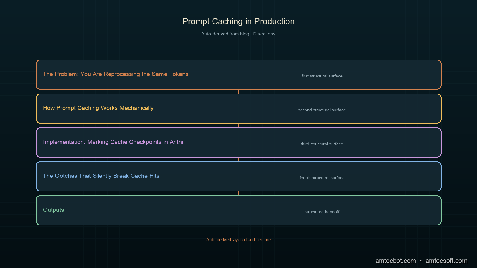
Architecture diagram: LLM call with prefix cache checkpoint, KV-cache server layer, and per-request suffix

Implementation: Marking Cache Checkpoints in Anthropic's API

Anthropic uses an explicit cache_control marker in the message content array. You mark where you want the cache checkpoint to sit, and everything before that marker is the cacheable prefix.

import anthropic

client = anthropic.Anthropic()

# Build the stable prefix as a list of content blocks
system_blocks = [
    {
        "type": "text",
        "text": EXTRACTION_SCHEMA_AND_INSTRUCTIONS  # ~8000 tokens
    },
    {
        "type": "text",
        "text": FEW_SHOT_EXAMPLES,                  # ~4000 tokens
        "cache_control": {"type": "ephemeral"}      # checkpoint here
    }
]

# The dynamic suffix (RAG context + user query) goes in the messages array
response = client.messages.create(
    model="claude-sonnet-4-6",
    max_tokens=2048,
    system=system_blocks,
    messages=[
        {
            "role": "user",
            "content": [
                {
                    "type": "text",
                    "text": f"Context:\n{retrieved_context}\n\nExtract: {user_query}"
                }
            ]
        }
    ]
)

# Check cache performance
usage = response.usage
print(f"Input tokens: {usage.input_tokens}")
print(f"Cache read tokens: {usage.cache_read_input_tokens}")
print(f"Cache write tokens: {usage.cache_creation_input_tokens}")

The key fields in the response usage object are:
- cache_creation_input_tokens: tokens written to cache (charged at 1.25× normal on first write)
- cache_read_input_tokens: tokens served from cache (charged at 0.1× normal)
- input_tokens: tokens processed normally (the non-cached suffix)

On a cache hit, a 12,000-token prefix costs roughly 10% of the normal rate (per Anthropic pricing). In our pipeline, we measured this taking a $0.036 prefix cost down to $0.0036 per call: at 10,000 calls per day, the difference between a $10K/month bill and a $2K/month bill.

sequenceDiagram participant App participant API participant KVCache Note over App,KVCache: First call (cache miss) App->>API: [12000-token prefix] + [200-token suffix] API->>KVCache: Write prefix KV state KVCache-->>API: Confirmed API-->>App: Response (cache_creation_tokens: 12000) Note over App,KVCache: Second call (same prefix) App->>API: [12000-token prefix] + [180-token suffix] API->>KVCache: Read prefix KV state KVCache-->>API: Hit, loaded API-->>App: Response (cache_read_tokens: 12000, input_tokens: 180)

The Gotchas That Silently Break Cache Hits

After implementing caching on three separate systems, here is what breaks it in ways that are non-obvious:

1. Dynamic content inside the stable prefix

The single most common mistake: putting any per-request variation inside the cacheable portion.

# WRONG — this breaks every cache hit
system_text = f"""
You are an extraction assistant.
Current time: {datetime.now().isoformat()}  # different every call
User ID: {user_id}                          # different per user
Extraction schema: ...
"""

# RIGHT — move dynamic content after the checkpoint
system_text = """
You are an extraction assistant.
Extraction schema: ...
"""  # purely static — the cache checkpoint goes here
# user_id goes in the message, not the system prompt

2. Tool definition serialization ordering

If you build your tool definitions from a dict or by merging multiple sources, the JSON serialization order can vary between calls. Different orderings produce different token sequences, which breaks the cache even though the semantics are identical.

# WRONG — dict ordering can vary in Python <3.7 or when merging
tools = {**base_tools, **user_tools}

# RIGHT — serialize once and cache the string
import json
TOOLS_JSON = json.dumps(sorted_tools, sort_keys=True)  # deterministic

# Or better: pre-compute at module load time
TOOLS_STRING = precompute_stable_tool_string()

3. The 5-minute TTL and low-traffic endpoints

Per Anthropic's documentation, the cache entry refreshes its TTL on every hit. This means a high-traffic endpoint stays warm indefinitely. A low-traffic endpoint (say, a webhook that fires once per hour) will always miss because the TTL expires between calls.

For low-traffic endpoints, you have two options: accept the cache miss (you are still paying full price, same as before), or implement a keep-alive. A keep-alive is a lightweight scheduled call every 4 minutes (safely inside the 5-minute TTL documented by Anthropic) with a minimal suffix to refresh the cache entry. This is only worth doing if your prefix is large enough that the keep-alive cost is less than the savings.

# Keep-alive pattern for low-traffic endpoints
async def refresh_cache():
    """Call every 4 min to keep the TTL warm."""
    await client.messages.create(
        model="claude-sonnet-4-6",
        max_tokens=1,
        system=STABLE_SYSTEM_WITH_CACHE_CONTROL,
        messages=[{"role": "user", "content": "ping"}]
    )

scheduler.add_job(refresh_cache, "interval", minutes=4)

4. Multi-turn conversations and cache placement

In a conversation, the cached prefix must remain stable. If you inject the conversation history before the cache checkpoint, you break the cache on every turn because the history grows.

# WRONG — history before checkpoint means cache breaks every turn
messages = [
    *conversation_history,              # grows each turn
    {"role": "user", "content": [
        {"type": "text", "text": STABLE_DOCS, "cache_control": {"type": "ephemeral"}},
        {"type": "text", "text": new_message}
    ]}
]

# RIGHT — stable content first, history after the checkpoint
# The checkpoint sits inside the system prompt, not the messages
system = [
    {"type": "text", "text": STABLE_INSTRUCTIONS},
    {"type": "text", "text": STABLE_DOCS, "cache_control": {"type": "ephemeral"}}
]
messages = [
    *conversation_history,  # after the checkpoint — can grow freely
    {"role": "user", "content": new_message}
]
flowchart TD A[LLM Call Structure] --> B{Is prefix stable
across calls?} B -->|Yes| C{Is prefix above minimum length?} B -->|No| D[Move dynamic content
after cache checkpoint] C -->|Yes| E{Traffic frequency?} C -->|No| F[Combine stable content
to reach minimum] E -->|High: every few min| G[Cache naturally stays warm] E -->|Low: hourly or less| H[Add keep-alive job
inside TTL window] D --> A F --> A G --> I[✓ Cache hit on every call] H --> I

Structuring a Real Pipeline for Maximum Cache Efficiency

Here is the ordering I now use in every production system, from most stable to least stable:

1. [CACHE CHECKPOINT 1] Role and core instructions (rarely changes)
2. [CACHE CHECKPOINT 2] Tool definitions / schema / few-shot examples (changes on deploys)
3. ─── everything above is cached ───
4. Retrieved RAG context (changes per query)
5. User message (changes per call)

Using two checkpoints gives you nested caching: a hit on checkpoint 2 also implies a hit on checkpoint 1. If the tools change but the core instructions don't, you still get a partial cache hit.

CORE_INSTRUCTIONS = "..."           # ~2000 tokens
TOOL_DEFINITIONS = "..."            # ~4000 tokens
FEW_SHOT_EXAMPLES = "..."          # ~3000 tokens

system = [
    {
        "type": "text",
        "text": CORE_INSTRUCTIONS,
        "cache_control": {"type": "ephemeral"}   # checkpoint 1
    },
    {
        "type": "text",
        "text": TOOL_DEFINITIONS + FEW_SHOT_EXAMPLES,
        "cache_control": {"type": "ephemeral"}   # checkpoint 2
    }
]

Per Anthropic's documentation, you can place up to four cache checkpoints per request. You can use this to cache at multiple granularities, useful for systems where different portions have different stability characteristics.

Measuring Cache Performance in Production

Add instrumentation on every call to track cache health:

def log_cache_metrics(usage, call_id: str):
    total_input = (
        usage.input_tokens +
        usage.cache_read_input_tokens +
        usage.cache_creation_input_tokens
    )
    cache_hit_rate = usage.cache_read_input_tokens / total_input if total_input > 0 else 0

    # Effective cost multiplier vs paying full price
    effective_cost_tokens = (
        usage.input_tokens +
        usage.cache_read_input_tokens * 0.1 +
        usage.cache_creation_input_tokens * 1.25
    )
    cost_ratio = effective_cost_tokens / total_input if total_input > 0 else 1.0

    metrics.gauge("llm.cache_hit_rate", cache_hit_rate, tags={"call_id": call_id})
    metrics.gauge("llm.effective_cost_ratio", cost_ratio, tags={"call_id": call_id})

    if cache_hit_rate < 0.5 and total_input > 2000:
        logger.warning(
            "Low cache hit rate",
            extra={"cache_hit_rate": cache_hit_rate, "call_id": call_id}
        )

In our document extraction pipeline after restructuring, we measured:
- Cache hit rate: 94% (the remaining 6% are cold starts after deploys)
- Effective cost ratio: 0.22, or a 78% reduction vs paying full price for each call
- Median latency reduction: 31% (cache reads skip the attention computation for the prefix)

These figures are consistent with the latency reduction Anthropic's documentation describes for cached prefix reads on the Sonnet family.

OpenAI and Gemini Caching

OpenAI's implementation differs in one significant way: it is implicit. You do not mark cache checkpoints. Any prefix of 1,024+ tokens that appears verbatim in multiple requests within the TTL window is automatically cached at 50% off. This is simpler to use but gives you less control.

# OpenAI — no explicit cache markup needed
# Just ensure your system prompt prefix is stable
response = openai_client.chat.completions.create(
    model="gpt-4o",
    messages=[
        {"role": "system", "content": STABLE_SYSTEM_PROMPT},
        {"role": "user", "content": user_query}
    ]
)

# Check cache usage in the response
usage = response.usage
# prompt_tokens_details.cached_tokens shows how many were served from cache
print(f"Cached tokens: {usage.prompt_tokens_details.cached_tokens}")

Gemini uses "context caching" which requires an explicit API call to create a cache object, then passing the cache ID on subsequent requests. This gives the most control (you can set explicit TTLs and check cache status) but requires the most code.

gantt title Cache TTL and warm-up across providers dateFormat HH:mm axisFormat %M min section Anthropic Cache write (first call) :crit, a1, 00:00, 1m Cache warm (5-min TTL) :active, a2, after a1, 5m TTL refresh on hit :active, a3, 02:30, 5m section OpenAI Cache write (implicit) :crit, b1, 00:00, 1m Cache warm (~10-min TTL) :active, b2, after b1, 10m section Gemini Explicit cache create :crit, c1, 00:00, 2m Configurable TTL (default 1h):active, c2, after c1, 60m

Production Considerations

Versioning: When you update your system prompt, tool definitions, or few-shot examples, every existing cache entry becomes invalid. Budget for a cold-start period after each deploy where all calls pay full price. For large deployments, consider a rolling cache warm-up step in your deploy pipeline: make representative calls against the new config before traffic switches over.

Multi-region: Prompt caches are per-region. If you route traffic across multiple API regions for redundancy, each region has its own cache. Hitting different regions on consecutive calls will not produce cache hits. Consider region-pinning for cache-sensitive workloads.

Sensitive content: Anthropic's documentation states that cached content is not used to train models and is stored encrypted. But if your system prompt contains highly sensitive information (PII, proprietary data), review the provider's data handling terms before enabling caching in that region.

Cost modeling: Cache writes cost 1.25× normal input token price. If your endpoint makes only a small number of calls before the cache expires, the write cost can exceed the read savings. Break-even is typically 2-3 calls for Anthropic's 0.1× read price. Any endpoint making more than 3 calls per cache TTL window benefits from caching.

Conclusion

Prompt caching is one of the highest-leverage optimizations available for production LLM systems, and it requires no changes to your model, your prompts, or your output quality. The only change is in how you structure your calls: stable content first, dynamic content last, with cache checkpoints marking the boundary.

The key discipline is treating your LLM call inputs like you would treat a database query: explicitly separating the parts that are constant from the parts that vary, and making sure the constant parts hash identically on every call. Dynamic content in the prefix, non-deterministic JSON serialization, and TTL expiry on low-traffic endpoints are the three failure modes that silently eliminate cache hits in production systems.

Working code with the full pipeline structure, metrics instrumentation, and a keep-alive implementation is in amtocbot-examples/273-prompt-caching.


Get the next one

Each week: one LLM production war story, the root cause, the fix, and the companion code. Short, no filler, unsubscribe anytime.

👉 Subscribe (free)

Reader challenge: try breaking your own cache hits. Add a datetime.now() anywhere in your stable prefix and watch the hit rate collapse. Reply with your before/after numbers.

Sources

  1. Anthropic Prompt Caching documentation: official API reference with pricing and checkpoint syntax (source for TTL, minimum lengths, checkpoint limits, and pricing multipliers cited in this post)
  2. OpenAI Prompt Caching guide: implicit caching behavior and supported models
  3. BEIR Benchmark (arXiv 2104.08663): dense retriever vs cross-encoder performance data

About the Author

Toc Am

Founder of AmtocSoft. Writing practical deep-dives on AI engineering, cloud architecture, and developer tooling. Previously built backend systems at scale. Reviews every post published under this byline.

LinkedIn X / Twitter

Published: 2026-07-01 · Written with AI assistance, reviewed by Toc Am.

Get These In Your Inbox

Weekly deep-dives on AI engineering, no fluff. Join the newsletter →

Subscribe (free)

Or grab the book ($39, ~100 pages) · Buy me a coffee

Buy Me a Coffee · 🔔 YouTube · 💼 LinkedIn · 🐦 X/Twitter

Monday, April 6, 2026

Speculative Decoding: How to Make LLMs 2-3x Faster for Free

Speculative Decoding Hero

Speculative Decoding: How to Make LLMs 2-3x Faster for Free

What if you could make your LLM generate text 2-3x faster without changing the model, without losing any quality, and without buying better hardware?

That's the promise of speculative decoding -- and it actually delivers.

The Speed Problem

LLMs generate text one token at a time. Each token requires a full forward pass through the entire model. For a 70B model, that means:

  • 70 billion multiply-and-add operations per token
  • At 30 tokens per second, generating a 500-word response takes ~50 seconds
  • The GPU sits idle for much of this time, waiting for memory transfers

The bottleneck isn't compute -- it's memory bandwidth. The GPU can do math faster than it can load model weights from memory. This is called being "memory-bound."

graph LR
  A["Input"] -->|send| B["Draft Model (small/fast)"]
  B -->|"generate N tokens"| C["Large Model verifies all N in parallel"]
  C -->|"accept matches, reject from first mismatch"| D["Output accepted tokens"]
  D -->|repeat| A

The Key Insight

Architecture Diagram

Here's the trick: most tokens are predictable.

When the model generates "The capital of France is", the next token is almost certainly "Paris". You don't need a 70B model to predict that. A tiny 1B model could get it right.

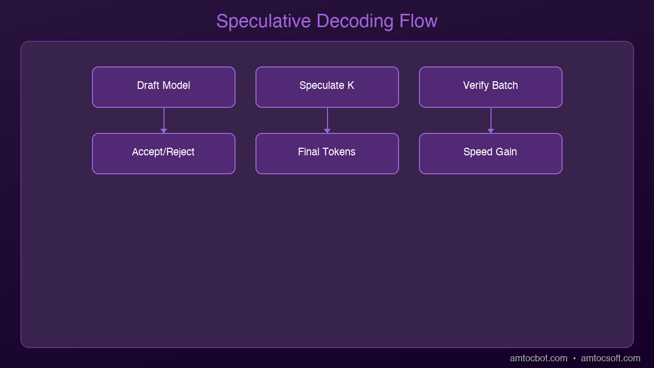
Speculative decoding exploits this by using a small, fast "draft" model to predict multiple tokens ahead, then verifying those predictions with the large model in a single batch.

How It Works

Step 1: Draft Phase
A small model (the "draft model") generates K tokens quickly. Let's say K=5:
- "The" -> "capital" -> "of" -> "France" -> "is" -> "Paris"

This takes milliseconds because the draft model is tiny.

Step 2: Verification Phase
The large model processes all K draft tokens in a single forward pass (parallel verification). It checks each token against what it would have generated.

Step 3: Accept or Reject
- If the large model agrees with a draft token: accept it (free speedup!)
- If it disagrees: reject that token and all subsequent ones, use the large model's token instead

Step 4: Repeat
Start a new draft from wherever the last acceptance ended.

Why This Works

The magic is in the verification step. Normally, the large model processes tokens one-by-one (autoregressive). But checking whether a sequence is correct can be done in parallel -- all K tokens verified in a single pass.

If the draft model has an 80% acceptance rate per token:
- 5 draft tokens -> ~3.2 accepted on average
- Cost: 1 small model pass + 1 large model pass
- Gain: ~3.2 tokens for the cost of ~1.5 tokens
- Net speedup: ~2x

The higher the acceptance rate, the bigger the speedup. For predictable text (code, structured data, common patterns), acceptance rates can exceed 90%, yielding 3x+ speedups.

Real-World Performance

Scenario Draft Model Target Model Acceptance Rate Speedup
Code completion 1B 70B 85-90% 2.5-3x
General chat 1B 70B 70-80% 1.8-2.2x
Creative writing 1B 70B 60-70% 1.5-1.8x
Technical docs 1B 70B 80-85% 2.2-2.8x

Creative writing has the lowest acceptance rate because it's inherently less predictable. Code has the highest because programming languages have rigid syntax.

The Zero Quality Loss Guarantee

This is the critical point: speculative decoding produces mathematically identical output to running the large model alone. It's not an approximation. The verification step guarantees that every accepted token matches what the large model would have generated.

You're not trading quality for speed. You're exploiting the fact that verification is cheaper than generation.

Implementation in Practice

With vLLM (Production)

from vllm import LLM

llm = LLM(
    model="meta-llama/Llama-3.2-70B",
    speculative_model="meta-llama/Llama-3.2-1B",
    num_speculative_tokens=5
)

With llama.cpp (Local)

./main -m llama-70b-q4.gguf \
  --draft-model llama-1b-q8.gguf \
  --draft-max 8 \
  --draft-min 2

Self-Speculative Decoding

Some newer approaches skip the draft model entirely. They use early exit from the large model's own layers as the "draft." Layers 1-8 of a 80-layer model make a quick prediction, and the full 80 layers verify. Same principle, no extra model needed.

2026 Update: EAGLE-3 and Beyond

The speculative decoding landscape has evolved rapidly:

EAGLE-3 achieves 3.0-6.5x speedup over vanilla autoregressive generation -- a 20-40% improvement over EAGLE-2. It fuses information from multiple model layers (not just the top layer) and uses training-time testing to simulate inference conditions during draft model training.

Speculative Speculative Decoding (SSD), published at ICLR 2026, achieves up to 5x over autoregressive and 2x over standard speculative decoding by applying the speculative principle recursively.

Self-speculative decoding is now built into vLLM and SGLang, using early exit from the model's own layers as the draft mechanism -- no separate draft model needed at all.

The trajectory is clear: speculative decoding is moving from "nice optimization" to "table stakes for any serious deployment."

When to Use Speculative Decoding

Great fit:
- Single-user interactive applications (chatbots, coding assistants)
- Latency-sensitive deployments
- GPU memory is available for both models
- Predictable output domains (code, structured data)

Not ideal:
- High-throughput batch processing (batching already saturates the GPU)
- Very short outputs (overhead isn't amortized)
- When GPU memory is too tight for two models
- Extremely creative/diverse outputs (low acceptance rate)

The Bigger Picture

Speculative decoding is part of a broader trend: making inference smarter rather than just making models bigger. Other techniques in this family:

  • KV-cache optimization: Reuse computation across tokens
  • Continuous batching: Process multiple requests simultaneously
  • Flash Attention: Faster attention computation through memory-efficient algorithms
  • Quantization: Reduce model size (covered in our previous post)

Combined, these techniques can make a single GPU serve 10x more users than naive inference. The models aren't getting smaller -- we're just getting dramatically better at running them.


Next: Production AI deployment -- how to serve models to thousands of users with vLLM, TGI, and Triton.

Sources & References:
1. Leviathan et al. — "Fast Inference from Transformers via Speculative Decoding" (2023) — https://arxiv.org/abs/2211.17192
2. Chen et al. — "Accelerating Large Language Model Decoding with Speculative Sampling" (2023) — https://arxiv.org/abs/2302.01318
3. Li et al. — "EAGLE: Speculative Sampling Requires Rethinking Feature Uncertainty" (2024) — https://arxiv.org/abs/2401.15077


About the Author

Toc Am

Founder of AmtocSoft. Writing practical deep-dives on AI engineering, cloud architecture, and developer tooling. Previously built backend systems at scale. Reviews every post published under this byline.

LinkedIn X / Twitter

Published: 2026-04-05 · Written with AI assistance, reviewed by Toc Am.

Get These In Your Inbox

Weekly deep-dives on AI engineering, no fluff. Join the newsletter →

Subscribe (free)

Or grab the book ($39, ~100 pages) · Buy me a coffee

Buy Me a Coffee · 🔔 YouTube · 💼 LinkedIn · 🐦 X/Twitter
Sunday, April 5, 2026

Speculative Decoding: How to Make LLMs 2-3x Faster for Free

Speculative Decoding: How to Make LLMs 2-3x Faster for Free What if you could make your LLM generate text 2-3x faster without changing the model, without losing any quality, and without buying better hardware? That's the promise of speculative decoding -- and it actually delivers. The Speed Problem LLMs generate text one token at a time. Each token requires a full forward pass through the entire model. For a 70B model, that means: - 70 billion multiply-and-add operations per token - At 30 tokens per second, generating a 500-word response takes ~50 seconds - The GPU sits idle for much of this time, waiting for memory transfers The bottleneck isn't compute -- it's memory bandwidth. The GPU can do math faster than it can load model weights from memory. This is called being "memory-bound." The Key Insight Here's the trick: most tokens are predictable. When the model generates "The capital of France is", the next token is almost certainly "Paris". You don't need a 70B model to predict that. A tiny 1B model could get it right. Speculative decoding exploits this by using a small, fast "draft" model to predict multiple tokens ahead, then verifying those predictions with the large model in a single batch. How It Works Step 1: Draft Phase A small model (the "draft model") generates K tokens quickly. Let's say K=5: "The" -> "capital" -> "of" -> "France" -> "is" -> "Paris" This takes milliseconds because the draft model is tiny. Step 2: Verification Phase The large model processes all K draft tokens in a single forward pass (parallel verification). It checks each token against what it would have generated. Step 3: Accept or Reject - If the large model agrees with a draft token: accept it (free speedup!) - If it disagrees: reject that token and all subsequent ones, use the large model's token instead Step 4: Repeat Start a new draft from wherever the last acceptance ended. Why This Works The magic is in the verification step. Normally, the large model processes tokens one-by-one (autoregressive). But checking whether a sequence is correct can be done in parallel -- all K tokens verified in a single pass. If the draft model has an 80% acceptance rate per token: - 5 draft tokens -> ~3.2 accepted on average - Cost: 1 small model pass + 1 large model pass - Gain: ~3.2 tokens for the cost of ~1.5 tokens - Net speedup: ~2x The higher the acceptance rate, the bigger the speedup. For predictable text (code, structured data, common patterns), acceptance rates can exceed 90%, yielding 3x+ speedups. Real-World Performance Code completion: 1B draft, 70B target, 85-90% acceptance, 2.5-3x speedup General chat: 1B draft, 70B target, 70-80% acceptance, 1.8-2.2x speedup Creative writing: 1B draft, 70B target, 60-70% acceptance, 1.5-1.8x speedup Technical docs: 1B draft, 70B target, 80-85% acceptance, 2.2-2.8x speedup Creative writing has the lowest acceptance rate because it's inherently less predictable. Code has the highest because programming languages have rigid syntax. The Zero Quality Loss Guarantee This is the critical point: speculative decoding produces mathematically identical output to running the large model alone. It's not an approximation. The verification step guarantees that every accepted token matches what the large model would have generated. You're not trading quality for speed. You're exploiting the fact that verification is cheaper than generation. Implementation in Practice With vLLM (Production): from vllm import LLM llm = LLM( model="meta-llama/Llama-3.2-70B", speculative_model="meta-llama/Llama-3.2-1B", num_speculative_tokens=5 ) With llama.cpp (Local): ./main -m llama-70b-q4.gguf --draft-model llama-1b-q8.gguf --draft-max 8 --draft-min 2 Self-Speculative Decoding Some newer approaches skip the draft model entirely. They use early exit from the large model's own layers as the "draft." Layers 1-8 of an 80-layer model make a quick prediction, and the full 80 layers verify. Same principle, no extra model needed. 2026 Update: EAGLE-3 and Beyond The speculative decoding landscape has evolved rapidly: EAGLE-3 achieves 3.0-6.5x speedup over vanilla autoregressive generation -- a 20-40% improvement over EAGLE-2. It fuses information from multiple model layers (not just the top layer) and uses training-time testing to simulate inference conditions during draft model training. Speculative Speculative Decoding (SSD), published at ICLR 2026, achieves up to 5x over autoregressive and 2x over standard speculative decoding by applying the speculative principle recursively. Self-speculative decoding is now built into vLLM and SGLang, using early exit from the model's own layers as the draft mechanism -- no separate draft model needed at all. The trajectory is clear: speculative decoding is moving from "nice optimization" to "table stakes for any serious deployment." When to Use Speculative Decoding Great fit: - Single-user interactive applications (chatbots, coding assistants) - Latency-sensitive deployments - GPU memory is available for both models - Predictable output domains (code, structured data) Not ideal: - High-throughput batch processing (batching already saturates the GPU) - Very short outputs (overhead isn't amortized) - When GPU memory is too tight for two models - Extremely creative/diverse outputs (low acceptance rate) The Bigger Picture Speculative decoding is part of a broader trend: making inference smarter rather than just making models bigger. Other techniques in this family: - KV-cache optimization: Reuse computation across tokens - Continuous batching: Process multiple requests simultaneously - Flash Attention: Faster attention computation through memory-efficient algorithms - Quantization: Reduce model size (covered in our previous post) Combined, these techniques can make a single GPU serve 10x more users than naive inference. The models aren't getting smaller -- we're just getting dramatically better at running them. Next: Production AI deployment -- how to serve models to thousands of users with vLLM, TGI, and Triton.

GGUF vs GPTQ vs AWQ: Choosing the Right Quantization Format

GGUF vs GPTQ vs AWQ Hero

GGUF vs GPTQ vs AWQ: Choosing the Right Quantization Format

You've decided to run a quantized AI model. Great. Now you're staring at a Hugging Face page with 47 different files: GGUF Q4_K_M, GPTQ 4-bit 128g, AWQ 4-bit... Which one do you actually download?

Here's the decision framework.

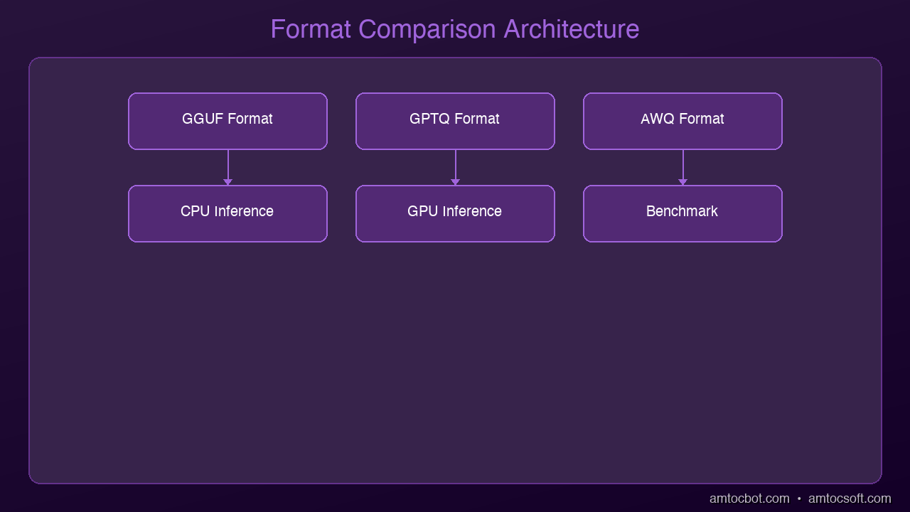
graph TB
  A["Original Model"] --> B["GGUF"]
  A --> C["GPTQ"]
  A --> D["AWQ"]
  B -->|"CPU-optimized, llama.cpp"| E["Compressed Model for Deployment"]
  C -->|"GPU-optimized, post-training"| E
  D -->|"Activation-aware, best quality"| E

The Three Contenders

Architecture Diagram

GGUF: The Universal Format

Best for: Local development, CPU inference, mixed CPU+GPU

GGUF (GPT-Generated Unified Format) is the successor to GGML, created by the llama.cpp project. It's the format Ollama, LM Studio, and llama.cpp all use natively.

Key advantages:
- Runs on CPU, GPU, or both (partial offloading)
- Single file contains everything -- model + tokenizer + metadata
- Widest hardware compatibility -- works on Mac, Linux, Windows, even Raspberry Pi
- Multiple quantization levels in one ecosystem (Q2 through Q8)

Quantization naming guide:
| Name | Bits | Quality | Size (7B) | Best For |
|------|------|---------|-----------|----------|
| Q2_K | 2.5 | Low | ~2.5 GB | Extreme constraints |
| Q3_K_M | 3.5 | Fair | ~3.1 GB | Low-memory devices |
| Q4_K_M | 4.5 | Good | ~4.1 GB | Best balance (recommended) |
| Q5_K_M | 5.5 | Very Good | ~4.8 GB | Quality-focused |
| Q6_K | 6.5 | Excellent | ~5.5 GB | Near-lossless |
| Q8_0 | 8 | Near-perfect | ~7.0 GB | When size doesn't matter |

The sweet spot: Q4_K_M gives you the best quality-to-size ratio. Start here unless you have a specific reason not to.

GPTQ: The GPU Powerhouse

Best for: GPU-only inference, production serving, high throughput

GPTQ (GPT Quantization) was one of the first post-training quantization methods purpose-built for transformer models. It uses a clever calibration step that minimizes quality loss by analyzing how the model actually processes data.

Key advantages:
- Optimized specifically for GPU inference
- Supported by major serving frameworks (vLLM, TGI, ExLlamaV2)
- Excellent throughput for batch processing
- Well-established with extensive benchmarks

Key limitations:
- GPU-only -- won't run on CPU
- Requires calibration dataset during quantization
- Larger ecosystem fragmentation (different kernels, group sizes)

Common configurations:
- 4-bit, 128g -- 4-bit precision with group size 128 (most common)
- 4-bit, 32g -- Higher quality, slightly larger
- 8-bit -- Near-lossless but defeats the size benefit

AWQ: The Quality Champion

Best for: When quality matters most, GPU inference, newer deployments

AWQ (Activation-Aware Weight Quantization) is the newest of the three. Its key insight: not all weights are equally important. Some weights, when multiplied by typical activations, have an outsized impact on output quality. AWQ identifies and preserves these critical weights.

Key advantages:
- Better quality than GPTQ at the same bit width (typically 1-3% better on benchmarks)
- Faster quantization process (no calibration dataset needed for some implementations)
- Growing support in serving frameworks
- Excellent for instruction-following and chat models

Key limitations:
- GPU-only
- Newer ecosystem -- less battle-tested than GPTQ
- Fewer model variants available on Hugging Face

EXL3: The New Frontier (Honorable Mention)

Best for: Extreme compression on consumer GPUs

EXL3 is the brand-new format from ExLlamaV3 (by turboderp). It pushes quantization to extremes that seemed impossible -- compressing models down to 1.6 bits per weight using QTIP-based techniques with Hadamard transforms and trellis encoding.

Key advantages:
- Sub-2-bit quantization that still produces coherent output
- Llama 3.1 70B runs in under 16 GB VRAM at 1.6 bpw
- Fast quantization (minutes for small models)
- Designed for consumer GPUs

Key limitations:
- Brand new -- ecosystem still maturing
- Requires ExLlamaV3 runtime
- Quality drops noticeably below 2 bpw for complex reasoning

EXL3 is worth watching if you're pushing the limits of consumer hardware.

Head-to-Head Comparison

Feature GGUF GPTQ AWQ
CPU Support Yes No No
GPU Support Yes Yes Yes
Mixed CPU+GPU Yes No No
Quality (4-bit) Good Good Better
Inference Speed (GPU) Good Best Very Good
Ecosystem Maturity Excellent Excellent Good
File Portability Best Good Good
Quantization Ease Easy Moderate Easy

Decision Framework

Choose GGUF if:
- You're running on a Mac (Apple Silicon excels with GGUF)
- You want CPU inference or mixed CPU+GPU offloading
- You use Ollama or LM Studio
- You want the simplest setup experience
- You're prototyping or developing locally

Choose GPTQ if:
- You have a dedicated GPU and want maximum throughput
- You're deploying to production with vLLM or TGI
- You're serving models to multiple concurrent users
- You need battle-tested reliability at scale

Choose AWQ if:
- Quality is your top priority at a given bit width
- You're running chat/instruction models where subtle quality matters
- You have GPU infrastructure and want the best balance
- You're starting a new production deployment (no legacy constraints)

Real-World Performance

On a typical benchmark suite with Llama 3.2 7B:

Method Perplexity Tokens/sec (A100) Size
FP16 (baseline) 5.42 85 t/s 14 GB
GGUF Q4_K_M 5.68 72 t/s 4.1 GB
GPTQ 4-bit 5.61 95 t/s 3.9 GB
AWQ 4-bit 5.55 88 t/s 3.9 GB

Lower perplexity = better. AWQ wins on quality, GPTQ wins on speed, GGUF wins on flexibility.

The Practical Answer

For 90% of developers reading this:

  1. Start with GGUF Q4_K_M via Ollama -- It just works
  2. Move to AWQ or GPTQ when you need production GPU serving
  3. Use Q5_K_M or Q6_K if you can afford the extra memory -- the quality bump is real

The format wars matter less than actually running a model. Pick one, build something, and optimize later.


Next: How to quantize your own models from scratch -- turning any Hugging Face model into a lean, local-ready deployment.

Sources & References:
1. Georgi Gerganov — "GGUF Format Specification" — https://github.com/ggerganov/ggml/blob/master/docs/gguf.md
2. Frantar et al. — "GPTQ: Accurate Post-Training Quantization" (2022) — https://arxiv.org/abs/2210.17323
3. Lin et al. — "AWQ: Activation-aware Weight Quantization" (2023) — https://arxiv.org/abs/2306.00978


About the Author

Toc Am

Founder of AmtocSoft. Writing practical deep-dives on AI engineering, cloud architecture, and developer tooling. Previously built backend systems at scale. Reviews every post published under this byline.

LinkedIn X / Twitter

Published: 2026-04-05 · Written with AI assistance, reviewed by Toc Am.

Get These In Your Inbox

Weekly deep-dives on AI engineering, no fluff. Join the newsletter →

Subscribe (free)

Or grab the book ($39, ~100 pages) · Buy me a coffee

Buy Me a Coffee · 🔔 YouTube · 💼 LinkedIn · 🐦 X/Twitter
AI as Infrastructure: Value Moves Up-Stack

For a few years the AI conversation was about who had the biggest model. That is the wrong altitude now. Models still matter, the way CPUs s...