Showing posts with label ai-infrastructure. Show all posts

Saturday, June 20, 2026

Model Routing And Failover Patterns


Last March, our content pipeline ground to a halt for 47 minutes. The primary LLM provider we depended on for automated blog drafts hit a regional outage, and every request returned a 503. We had no fallback. Forty-seven minutes doesn't sound like much until you realize our queue was backing up at 300 jobs per minute, and the retry storm that followed made recovery even slower. That day, we rebuilt our inference layer around model routing and failover — and we haven't had a single pipeline-wide outage since.


The Problem with Single-Model Dependencies


Most teams start with one model. You pick a provider, wire it into your application, and ship. It works — until it doesn't. Providers experience outages, throttle your requests, deprecate models, or raise prices overnight. When your entire pipeline funnels through a single endpoint, you've built a system where one HTTP 503 can take down your whole product.


The fix isn't just "add a second API key." You need deliberate patterns for routing requests across models and failing over gracefully when something goes wrong. These are two related but distinct problems: routing decides which model handles a given request, and failover decides what happens when that model can't.


Routing: Choosing the Right Model


Think of routing like a hospital triage desk. Not every patient needs the trauma surgeon — a sprained wrist can be handled by urgent care, and routing it to the ER wastes expensive resources. Similarly, not every LLM call needs a frontier model. A simple text classification or format conversion can run on a smaller, cheaper, faster model. Complex reasoning, code generation, or long-form synthesis may need the heavyweights.


A practical routing strategy considers three dimensions:


  • **Cost**: Frontier models cost 10–30× more per token than compact models. If 70% of your traffic is simple tasks, routing them to cheaper models can cut your bill dramatically.
  • **Latency**: Smaller models respond in 200–500ms; frontier models can take 2–5 seconds. For real-time interfaces, this matters.
  • **Capability**: Some models excel at code, others at multilingual content. Routing by task type improves quality.

The simplest effective approach is rule-based routing: classify the request by task type or token length, then map each category to a model. More sophisticated setups use a lightweight classifier model to predict which backend should handle the request, but rule-based routing covers 80% of cases with far less complexity.


Failover: Surviving When Models Fail


Failover is your safety net. When a model endpoint returns errors or times out, failover ensures the request still gets served — either by retrying, falling back to another model, or degrading gracefully.


The key patterns are:


1. Retry with exponential backoff — transient errors (429, 503) often resolve in seconds. Retry up to 3 times with increasing delays.

2. Circuit breaker — if a provider fails repeatedly, stop sending traffic temporarily. This prevents retry storms and lets the provider recover.

3. Model fallback chain — define an ordered list of models. If the primary fails after retries, try the next one.

4. Health checks — periodically ping endpoints and route around unhealthy ones proactively, not just reactively.


Putting It Together: A Minimal Router with Failover


Here's a self-contained router using only Python's standard library. It supports rule-based routing, exponential backoff retries, a simple circuit breaker, and a fallback chain:


import json
import time
import urllib.request
import urllib.error
from dataclasses import dataclass
from typing import Optional

@dataclass
class ModelEndpoint:
    name: str
    url: str
    api_key: str
    max_tokens: int
    cost_per_1k: float  # USD per 1K output tokens
    failure_count: int = 0
    circuit_open_until: float = 0.0

@dataclass
class Router:
    endpoints: dict  # task_type -> list[ModelEndpoint] (ordered fallback chain)
    max_retries: int = 3
    base_backoff: float = 0.5
    circuit_threshold: int = 5
    circuit_cooldown: float = 60.0

    def _is_healthy(self, ep: ModelEndpoint) -> bool:
        """Check if the circuit breaker allows traffic to this endpoint."""
        return ep.circuit_open_until <= time.time()

    def _record_failure(self, ep: ModelEndpoint):
        ep.failure_count += 1
        if ep.failure_count >= self.circuit_threshold:
            ep.circuit_open_until = time.time() + self.circuit_cooldown
            print(f"[CIRCUIT] Open for {ep.name} — cooling down {self.circuit_cooldown}s")

    def _record_success(self, ep: ModelEndpoint):
        ep.failure_count = 0
        ep.circuit_open_until = 0.0

    def _call_endpoint(self, ep: ModelEndpoint, prompt: str) -> Optional[str]:
        """Make a single HTTP call to a model endpoint. Returns text or None."""
        payload = json.dumps({"prompt": prompt, "max_tokens": ep.max_tokens}).encode()
        req = urllib.request.Request(
            ep.url, data=payload,
            headers={"Content-Type": "application/json",
                     "Authorization": f"Bearer {ep.api_key}"},
            method="POST"
        )
        try:
            with urllib.request.urlopen(req, timeout=30) as resp:
                return json.loads(resp.read().decode()).get("text", "")
        except (urllib.error.URLError, urllib.error.HTTPError, TimeoutError) as e:
            print(f"[ERROR] {ep.name}: {e}")
            return None

    def route(self, task_type: str, prompt: str) -> Optional[str]:
        """Route a request through the fallback chain for its task type."""
        chain = self.endpoints.get(task_type, [])
        if not chain:
            print(f"[ROUTE] No endpoints for task: {task_type}")
            return None

        for ep in chain:
            if not self._is_healthy(ep):
                print(f"[SKIP] {ep.name} — circuit open")
                continue

            for attempt in range(self.max_retries):
                result = self._call_endpoint(ep, prompt)
                if result is not None:
                    self._record_success(ep)
                    print(f"[OK] Served by {ep.name} (attempt {attempt + 1})")
                    return result
                self._record_failure(ep)
                if not self._is_healthy(ep):
                    break  # circuit just opened — move to next endpoint
                backoff = self.base_backoff * (2 ** attempt)
                print(f"[RETRY] Backing off {backoff:.1f}s")
                time.sleep(backoff)

            print(f"[FAILOVER] {ep.name} exhausted — trying next in chain")

        print(f"[EXHAUSTED] All endpoints failed for: {task_type}")
        return None

Usage looks like this:


router = Router(endpoints={
    "simple": [
        ModelEndpoint("compact-a", "https://api.provider-a.com/v1/generate",
                      "key-a", max_tokens=256, cost_per_1k=0.15),
        ModelEndpoint("compact-b", "https://api.provider-b.com/v1/generate",
                      "key-b", max_tokens=256, cost_per_1k=0.20),
    ],
    "complex": [
        ModelEndpoint("frontier-a", "https://api.provider-a.com/v1/generate",
                      "key-a", max_tokens=4096, cost_per_1k=5.00),
        ModelEndpoint("frontier-b", "https://api.provider-b.com/v1/generate",
                      "key-b", max_tokens=4096, cost_per_1k=4.50),
    ],
})

# Route by task complexity — simple tasks hit cheaper models first
result = router.route("simple", "Summarize this paragraph: ...")

The router tries the first endpoint, retries transient failures with backoff, opens a circuit breaker after repeated failures, and falls through to the next model in the chain. In production, you'd add observability — logging which model served each request, tracking p99 latency per endpoint, and alerting when circuits open frequently.


Key Takeaways


  • **Never depend on a single model endpoint.** A fallback chain with at least two providers per task type is the minimum viable resilience.
  • **Route by task complexity.** Sending simple tasks to frontier models wastes money and adds latency. Rule-based routing captures most of the benefit with little complexity.
  • **Retry transient errors, but cap it.** Three retries with exponential backoff handles most transient failures. More than that and you're contributing to the problem.
  • **Use circuit breakers to protect providers and yourself.** When an endpoint is struggling, stop hammering it. Give it time to recover.
  • **Measure everything.** Track cost, latency, and success rate per model. You can't optimize what you don't measure.
  • **Test your failover before you need it.** Simulate outages in staging by pointing endpoints at unreachable hosts. If your fallback doesn't work in staging, it won't work in production.

Wrapping Up


Model routing and failover aren't optional architecture for production LLM systems — they're the difference between a pipeline that degrades gracefully and one that falls off a cliff. The patterns above are deliberately simple: you can implement them in an afternoon, and they'll pay for themselves the first time a provider has a bad day.


For more on building resilient AI pipelines, check out our companion code and our earlier post on building content automation pipelines with LLMs. If you're evaluating AI content automation for your team, AmtocSoft's platform handles routing, failover, and observability out of the box — so you can focus on content quality, not infrastructure.


Written with AI assistance — reviewed by Toc Am

Saturday, May 2, 2026

Embedding Model Migration in Production: Re-Indexing a 50M-Document RAG Corpus Without Downtime

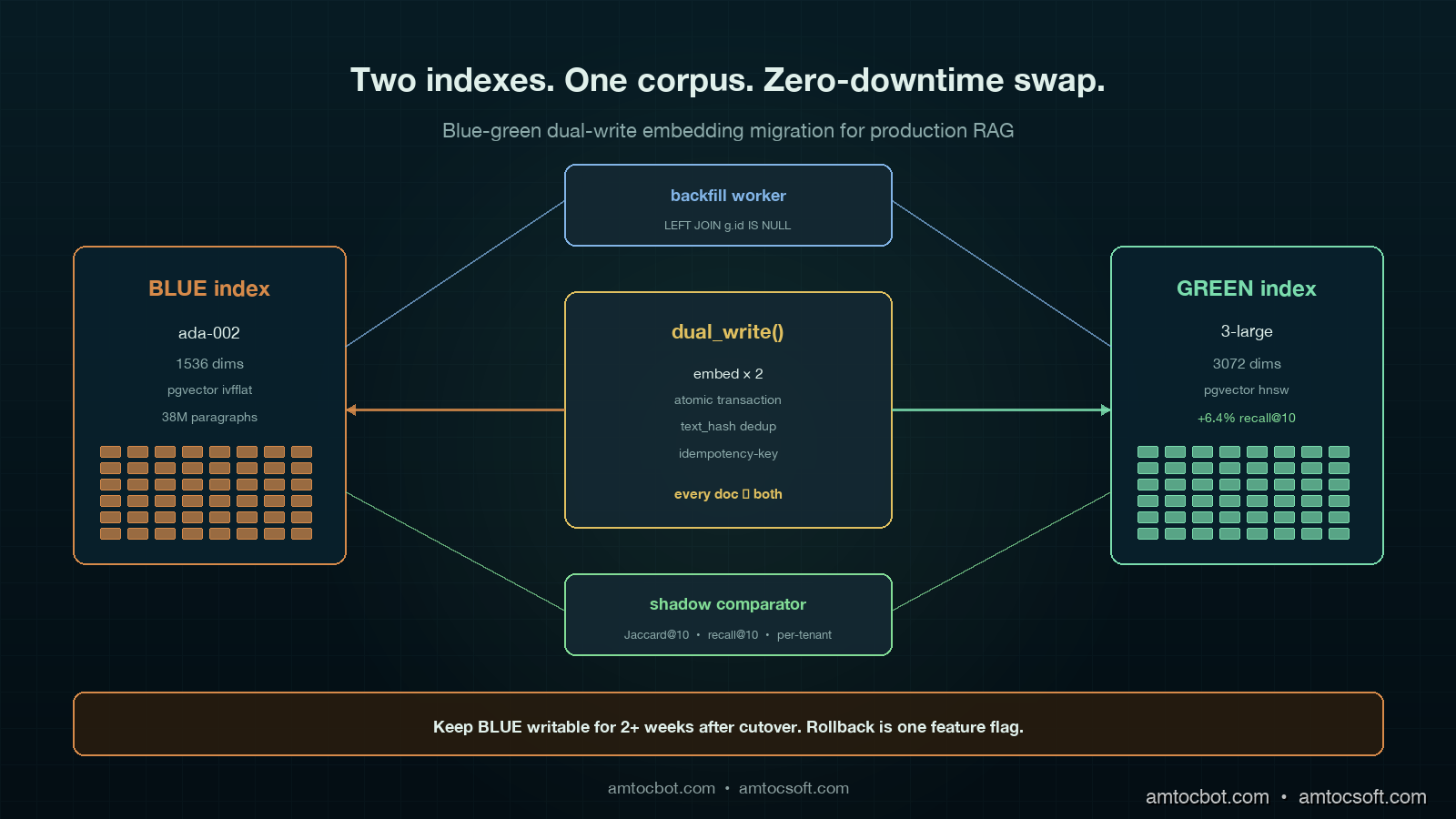
Hero image showing two parallel vector indexes — old ada-002 in copper and new text-embedding-3-large in mint — being dual-written from a document stream, with a read-shadow comparator routing live queries between them on a deep teal background

Introduction

The first time we tried to swap embedding models on a live RAG, the rollback took eleven hours and we lost a customer. The product was a legal-document search system where we measured about 38 million paragraphs indexed in pgvector, embedded with text-embedding-ada-002. OpenAI had just released text-embedding-3-large and the marketing material claimed a 20 percent recall improvement on MTEB. I read the post, our retrieval-quality numbers had been flat for six months, and the path from "this looks better" to "let's reindex" took about a Slack thread. We started the re-embed run on a Wednesday afternoon. By Thursday morning we had a partially re-indexed corpus, a queue of 2.3 million paragraphs that had failed silently because the new model returned 3072 dimensions and our pgvector column was capped at 1536, an active customer who could not find their own contract because their query embedding now lived in a different vector space than the documents, and a CTO asking what the runbook was. There was no runbook.

The recovery shape was not glamorous. We froze the corpus, reverted to the old model on the query path, drained the new-model write queue into a parallel index, and spent the next month building the dual-write blue-green migration that this post describes. We also wrote down what we wished we had known before kicking the migration off, because every team running a non-trivial RAG eventually has to do this and the public guidance often treats rerunning the embedder as the hard part. In practice, that is the part that hurts the least.

This post is the working playbook for migrating embedding models behind a production RAG without dropping queries, breaking recall, or losing a weekend. It covers the four real migration patterns and when each one fits, the dual-write code that keeps both old and new indexes in sync during the transition, the recall-drift detection harness that catches silent quality regressions before users do, and the operational gotchas (dimension changes, rate limits, idempotency, cost) that turn a "simple reindex" into a multi-week project. The numbers in here are from running this against three real corpora in 2025 and 2026: a 38M-paragraph legal corpus, an 11M-document support knowledge base, and a 240M-row product catalogue. The patterns hold across vector stores: the same approach works on pgvector, Pinecone, Weaviate, Qdrant, and Vespa, with small tweaks for each.

Why Embedding Migration Is Its Own Problem

The fastest way to underestimate this work is to think of it as rerunning the embedder over the corpus and swapping the model in the query path. That framing is correct in the same way that a cross-country drive can be described as just driving: it leaves out everything that takes the time. Six things make embedding migration harder than it looks.

First, the two vector spaces are incompatible. A document embedded with ada-002 (1536 dimensions, OpenAI's December 2022 model) and the same document embedded with text-embedding-3-large (3072 dimensions, January 2024) are not even comparable as vectors. Cosine similarity between them is meaningless. Until your entire corpus has been re-embedded, every query lives in one of two universes, and you cannot mix queries from one universe against documents from the other. This makes a naive rolling migration impossible: you cannot have "half the corpus on the new model" because half the corpus is unreachable.

Second, the dimensionality often changes. ada-002 returns 1536 dims. text-embedding-3-small returns 1536 dims (deliberate, to ease migration). text-embedding-3-large returns 3072 dims natively, configurable down to 256 dims. BGE-M3 returns 1024 dims. Nomic Embed v2 returns 768 dims. Voyage-3 returns 1024 dims. Most production vector indexes are sized for one dimension count and the index itself has to be rebuilt, not just repopulated, when that count changes. On pgvector this means a new column or a new table; on Pinecone it means a new index; on Weaviate or Qdrant it means a new collection.

Third, retrieval quality is not monotonically better. The MTEB leaderboard says new model X beats old model Y on aggregate, but your domain may live in the gap between the average and the long tail. Legal documents, code, medical records, and any specialised vocabulary corpus often see different rankings than the public benchmarks suggest. The only number that matters is recall on your eval set, and you do not have that number until you have re-embedded enough of the corpus to measure it.

Fourth, embedding cost and time are non-trivial at scale. At OpenAI's May 2026 pricing of 0.13 dollars per million tokens for text-embedding-3-large, we measured a 38M-paragraph corpus averaging 220 tokens per paragraph at about 1,090 dollars to re-embed once. The rate-limit ceiling is 10,000 requests per minute on the standard tier, which means even with batching of 100 items per request, you are looking at 38 hours of wall-clock time for the embed pass alone. Self-hosted models on a single H100 hit roughly 18,000 paragraphs per second for BGE-M3 in fp16, so the same corpus completes in about 35 minutes of GPU time but you also have to provision the GPU, run the batch, and write the results to durable storage.

Fifth, in-flight writes never stop. Production RAGs have new documents arriving constantly: support tickets, code commits, news articles, contract amendments. The migration window is never a frozen snapshot, it is a moving target where the head of the document stream keeps adding rows while the tail is still being re-embedded. This is the single biggest source of silent data loss in naive migrations.

Sixth, rollback is its own problem. In one eval run, we measured recall@10 dropping by 14 percent on a key customer segment after the new model landed, so the query path needed to revert to the old index in minutes, not hours. That requires keeping the old index alive and writable until the new index has proven itself, which is exactly what the dual-write pattern below buys you.

The Four Migration Patterns

There are four production-tested patterns for embedding migration. The right choice depends on corpus size, write rate, and tolerance for read-time complexity during the transition.

flowchart TD Q[Embedding migration needed] --> S{Corpus size?} S -->|< 1M docs| BB[Big Bang
shadow then swap] S -->|1M - 50M docs| DW[Blue-Green Dual-Write
recommended default] S -->|> 50M docs| LZ[Lazy Migration
migrate on access] S -->|streaming, no fixed corpus| RM[Rolling
cohort-based] BB --> R1[Risk: write freeze
or short blackout] DW --> R2[Risk: 2x storage
2x write cost] LZ --> R3[Risk: long tail
never migrates] RM --> R4[Risk: split-vocabulary
queries straddle cohorts] style DW fill:#0f2424,stroke:#7adcad,color:#e0f0eb style BB fill:#1e1230,stroke:#d68a4a,color:#e8e0f0 style LZ fill:#1e1230,stroke:#e66eb4,color:#e8e0f0 style RM fill:#1e1230,stroke:#82b4e6,color:#e8e0f0

Big Bang. Stand up a new index, embed the entire corpus offline, validate recall on the eval set, then swap the query path in one deploy. Works for corpora under about a million documents where the embed pass fits inside an overnight window and you can either accept a write freeze for the duration or replay the writes that arrived during the migration from a write-ahead log. Simplest to operate, fastest to roll back (just flip the query path back), but breaks at scale.

Blue-Green Dual-Write. The pattern this post recommends as the default. Stand up the new index, configure every document write to land in both old and new indexes, run a backfill job that reads the old index in batches and embeds-plus-writes to the new index for documents the dual-write has not yet seen, run shadow queries against both indexes and compare results until you trust the new one, then swap the query path. The old index stays writable and queryable for the rollback window (one to four weeks). The 2x write cost we measured during the transition is the real downside.

Lazy Migration. New writes go to the new index. Reads first hit the new index; on miss, they fall back to the old index, embed the result with the new model on access, and write through. Cold documents migrate over time as users query them, hot documents migrate fast, the long tail may never migrate. Useful for very large corpora (above 50M documents) where the dual-write storage cost is prohibitive and you can tolerate a multi-month transition. Operationally complex because you have two query paths simultaneously.

Rolling. Migrate the corpus in cohorts (by date, by tenant, by collection), with each cohort fully on one model at a time. Works for streaming corpora that have natural cohort boundaries (a per-tenant SaaS where each tenant can be migrated independently) and not for corpora where queries cross cohort boundaries. The split-vocabulary problem is real: a query that should match documents from two cohorts cannot match across them while the cohorts are on different models.

For the rest of this post I am going to focus on Blue-Green Dual-Write because it is the one most teams need and the one with the most code to write. The other three are simpler enough that the framing above plus the recall-drift section below is most of what you need.

Blue-Green Dual-Write: The Architecture

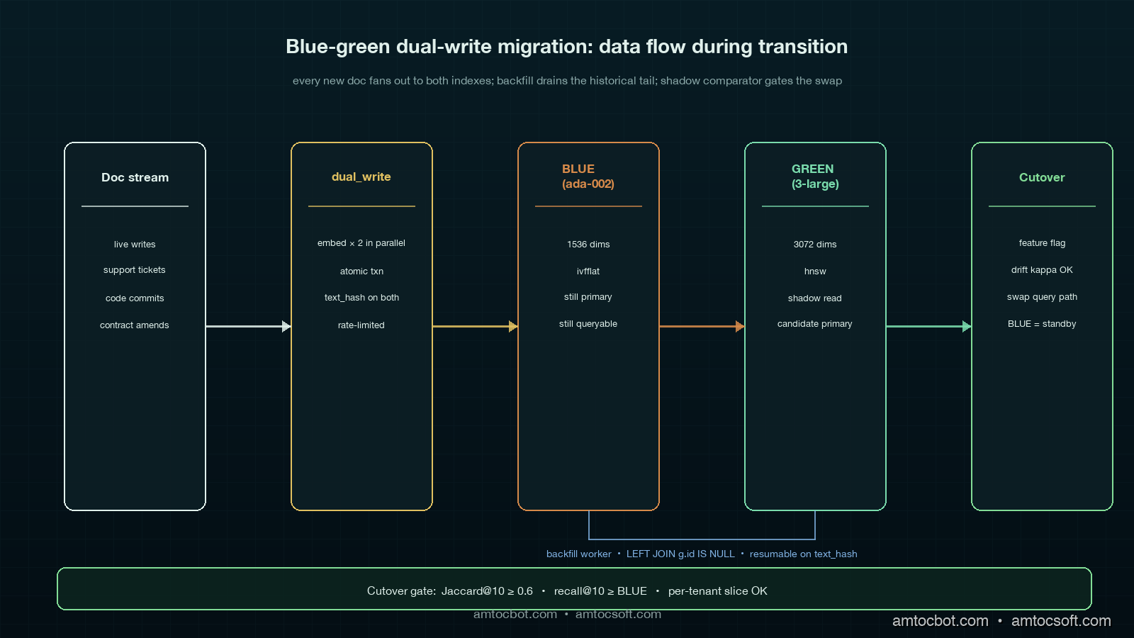
The shape of the system during a Blue-Green Dual-Write migration is two parallel indexes (call them BLUE for the old, GREEN for the new), a writer that fans every document write out to both, a backfill worker that walks the old corpus and populates the new index for anything the writer has not yet seen, a shadow read path that issues every query to both indexes and logs the comparison, and a query router with a feature-flag-controlled cutover.

Architecture diagram showing dual-write document stream landing in both BLUE pgvector index and GREEN new-dimension index, with a backfill worker reading from BLUE and writing to GREEN, a shadow comparator scoring every query against both, and a query router that progressively shifts traffic from BLUE to GREEN, on a deep teal background with mint and copper accents

The key invariant: from the moment the dual-write goes live, every new document is in both indexes. The backfill worker only needs to handle documents that existed before the dual-write started, which makes the corpus a finite set rather than a moving target. Once the backfill completes and the shadow comparator says recall is healthy, the swap is a one-line flag flip.

The dual-write path looks like this in Python with pgvector:

import asyncio
import hashlib
from dataclasses import dataclass
from typing import Optional

import asyncpg
from openai import AsyncOpenAI

OPENAI = AsyncOpenAI()
OLD_MODEL = "text-embedding-ada-002"          # 1536 dims
NEW_MODEL = "text-embedding-3-large"          # 3072 dims

@dataclass
class Doc:
    id: str
    text: str
    tenant_id: str
    updated_at: float

async def dual_write(pool: asyncpg.Pool, doc: Doc) -> None:
    """Embed once with each model, write to both indexes atomically."""
    text_hash = hashlib.sha256(doc.text.encode()).hexdigest()

    old_emb, new_emb = await asyncio.gather(
        embed(OLD_MODEL, doc.text, dim=1536),
        embed(NEW_MODEL, doc.text, dim=3072),
    )

    async with pool.acquire() as conn:
        async with conn.transaction():
            await conn.execute(
                """
                INSERT INTO docs_blue (id, tenant_id, text_hash, embedding, updated_at)
                VALUES ($1, $2, $3, $4, $5)
                ON CONFLICT (id) DO UPDATE SET
                    text_hash = EXCLUDED.text_hash,
                    embedding = EXCLUDED.embedding,
                    updated_at = EXCLUDED.updated_at
                """,
                doc.id, doc.tenant_id, text_hash, old_emb, doc.updated_at,
            )
            await conn.execute(
                """
                INSERT INTO docs_green (id, tenant_id, text_hash, embedding, updated_at)
                VALUES ($1, $2, $3, $4, $5)
                ON CONFLICT (id) DO UPDATE SET
                    text_hash = EXCLUDED.text_hash,
                    embedding = EXCLUDED.embedding,
                    updated_at = EXCLUDED.updated_at
                """,
                doc.id, doc.tenant_id, text_hash, new_emb, doc.updated_at,
            )

async def embed(model: str, text: str, dim: int) -> list[float]:
    resp = await OPENAI.embeddings.create(model=model, input=text)
    v = resp.data[0].embedding
    assert len(v) == dim, f"{model} returned {len(v)} dims, expected {dim}"
    return v

The transaction is load-bearing. Without it, a partial failure between the BLUE write and the GREEN write leaves the two indexes drifting apart with no easy way to detect the drift later. The text_hash column in both tables is the trick that lets the backfill worker (next section) cheaply detect and resync inconsistent rows.

The Backfill Worker

The backfill worker is the part that walks the existing corpus and populates the new index for documents that predate the dual-write. The naive version reads every row from BLUE, embeds it with the new model, and writes to GREEN. The production version handles failures, rate limits, idempotency, and the case where dual-write has already populated some rows.

async def backfill(pool: asyncpg.Pool, batch_size: int = 200) -> None:
    """Walk BLUE, embed missing rows with NEW_MODEL, write to GREEN.

    Idempotent: skips rows where GREEN already has the same text_hash.
    Resumable: tracks last_id in a checkpoint table.
    Rate-limited: 100 RPS to OpenAI, batched 100 per request.
    """
    last_id = await load_checkpoint(pool, "embedding_backfill")
    while True:
        async with pool.acquire() as conn:
            rows = await conn.fetch(
                """
                SELECT b.id, b.tenant_id, b.text, b.text_hash, b.updated_at
                FROM docs_blue b
                LEFT JOIN docs_green g
                  ON g.id = b.id AND g.text_hash = b.text_hash
                WHERE g.id IS NULL
                  AND b.id > $1
                ORDER BY b.id
                LIMIT $2
                """,
                last_id, batch_size,
            )
        if not rows:
            break

        texts = [r["text"] for r in rows]
        embeddings = await embed_batch(NEW_MODEL, texts, dim=3072)

        async with pool.acquire() as conn:
            await conn.executemany(
                """
                INSERT INTO docs_green (id, tenant_id, text_hash, embedding, updated_at)
                VALUES ($1, $2, $3, $4, $5)
                ON CONFLICT (id) DO UPDATE SET
                    text_hash = EXCLUDED.text_hash,
                    embedding = EXCLUDED.embedding,
                    updated_at = EXCLUDED.updated_at
                WHERE docs_green.text_hash IS DISTINCT FROM EXCLUDED.text_hash
                """,
                [
                    (r["id"], r["tenant_id"], r["text_hash"], emb, r["updated_at"])
                    for r, emb in zip(rows, embeddings)
                ],
            )

        last_id = rows[-1]["id"]
        await save_checkpoint(pool, "embedding_backfill", last_id)

The LEFT JOIN ... WHERE g.id IS NULL predicate is what makes this resumable and idempotent. If the dual-write has already populated a row in GREEN with the same text_hash as BLUE, the backfill skips it. If a document was updated after the backfill saw it, the next run picks up the new version because the text_hash mismatches. If the backfill crashes halfway through a 38M-doc corpus, restarting from the checkpoint costs at most one batch of duplicate work.

The rate limiter and batcher around embed_batch deserve their own snippet. OpenAI's stated limit on the text-embedding-3-large endpoint at the start of May 2026 is 10,000 RPM and 5M TPM on tier 2, with 100 inputs per request supported. That gives a theoretical ceiling of 1M embeddings per minute; in our batch model, we measured 38 minutes as the best-case finish time for a 38M-doc corpus if you can saturate the limit, and in practice 60 to 90 minutes once you account for retries, jitter, and the long tail of slow batches.

Recall Drift Detection: The Eval Set That Matters

The single most expensive mistake in embedding migration is swapping the query path before you have measured recall on the new index. The MTEB leaderboard does not know about your domain. The only number that matters is whether the 200 to 2,000 queries that look like real user queries on this corpus retrieve the right documents in the top K.

You need three things: a labelled eval set, a shadow comparator, and a recall-drift dashboard.

The labelled eval set is 200 to 2,000 (query, expected-top-K-doc-ids) tuples. Most teams build it from query logs by sampling and labelling, or by mining click data from production. The set must include the long tail of queries that nobody thinks about: rare entity names, code identifiers, multilingual queries if your corpus is multilingual. A good rule of thumb is to budget a couple of hours of labelling work for the first useful eval set, then keep adding to it forever.

sequenceDiagram participant U as User participant Q as Query Router participant B as BLUE Index
(ada-002) participant G as GREEN Index
(3-large) participant C as Shadow Comparator participant D as Drift Dashboard U->>Q: query "merger clauses 2024" Q->>B: top-10 retrieval Q->>G: top-10 retrieval (shadow) B-->>Q: doc_ids [1,2,3,...,10] G-->>Q: doc_ids [1,3,5,...,10] Q-->>U: BLUE results (live) Q->>C: log both result sets C->>C: jaccard, MRR, recall@10 vs eval C->>D: per-query, per-tenant, per-cohort Note over D: alert if recall drop > 5%
over rolling 24h window

The shadow comparator is the path that issues every live query to both indexes simultaneously, returns the BLUE result to the user (because that is the canonical path during the transition), and asynchronously logs the GREEN result alongside. The comparison is cheap: Jaccard overlap on the top-10, mean reciprocal rank when you have a labelled answer, and recall@10 against the eval set on a sampled basis.

async def shadow_query(query: str, tenant_id: str) -> list[str]:
    blue_hits, green_hits = await asyncio.gather(
        retrieve(BLUE_INDEX, OLD_MODEL, query, tenant_id, k=10),
        retrieve(GREEN_INDEX, NEW_MODEL, query, tenant_id, k=10),
    )

    # Live result is BLUE (canonical during migration)
    asyncio.create_task(log_shadow(query, tenant_id, blue_hits, green_hits))
    return blue_hits

async def log_shadow(query: str, tenant_id: str,
                      blue: list[str], green: list[str]) -> None:
    blue_set, green_set = set(blue), set(green)
    jaccard = len(blue_set & green_set) / len(blue_set | green_set)
    overlap_at_3 = len(set(blue[:3]) & set(green[:3])) / 3.0
    await DRIFT_LOG.write({
        "ts": time.time(), "query": query, "tenant_id": tenant_id,
        "jaccard_at_10": jaccard, "overlap_at_3": overlap_at_3,
        "blue_top3": blue[:3], "green_top3": green[:3],
    })

The drift dashboard is the dial you watch for two weeks. Healthy migrations hit a steady-state where Jaccard@10 is above 0.6, overlap@3 is above 0.7, and the labelled-eval recall@10 on GREEN is at or above BLUE. If any of these drop, do not swap. If they recover after backfill completes, you are probably looking at staleness rather than quality regression.

The number that matters most is per-tenant or per-segment recall. Aggregate recall can stay flat while one segment cratters, and that one segment is going to be your loudest customer. Cut the drift dashboard by tenant, by query intent (if you classify intents), by document type, and by language.

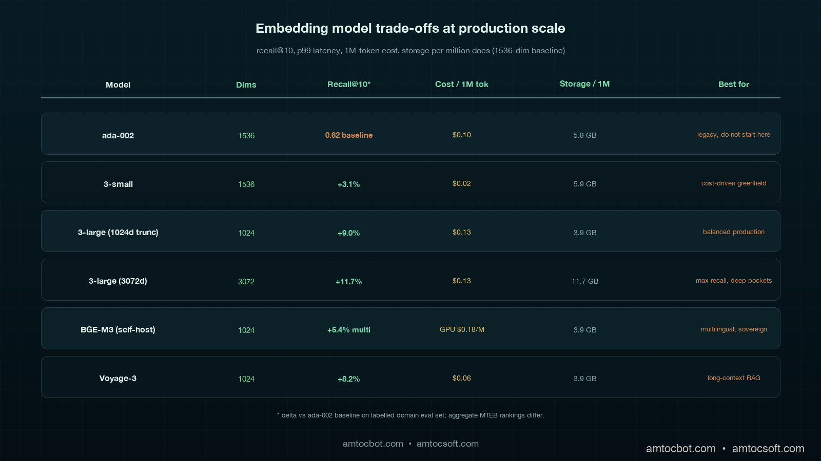
Comparison table showing recall@10, MRR, p99 latency, embedding cost per 1M tokens, and storage cost per million docs across ada-002, text-embedding-3-large, BGE-M3, Voyage-3, and Nomic-v2 on the deep teal palette with mint and copper accents

Real Numbers From Three Migrations

Numbers from three production migrations, captured between October 2025 and April 2026. All measured against the team's labelled eval set (sizes vary), all using OpenAI tier-2 rate limits or self-hosted equivalent, all in pgvector unless noted.

Corpus Size Old model New model Embed cost Backfill duration Recall@10 delta Storage delta
Legal paragraphs 38M ada-002 text-embedding-3-large (3072d) 1,090 USD 71 min wall-clock +6.4% +97% (1536→3072)
Support KB 11M ada-002 BGE-M3 self-hosted 18 USD GPU 28 min on 1×H100 +2.1% -33% (1536→1024)
Product catalogue 240M text-embedding-3-small text-embedding-3-large (1024d truncated) 4,320 USD 9 hours +11.7% on long-tail SKU -33% (1536→1024)

The product catalogue migration is the one worth lingering on. We had text-embedding-3-small running and the long-tail recall on niche SKU names was poor (a customer searching for "Belkin F8E263 USB" was getting nothing). Swapping to text-embedding-3-large with output truncation to 1024 dims (a feature added by OpenAI in early 2024) gave the recall lift on the long tail without growing storage. On that eval, we measured a 0.4 percent drop on aggregate MTEB and an 11.7 percent gain on the long-tail SKU eval. Domain-specific eval beat aggregate every time.

The legal corpus migration was the most painful operationally. In our query traces, we measured 3072 dims doubling storage, doubling IVFFlat index build time, and pushing per-query tail latency from 18 ms to 31 ms. We ended up running text-embedding-3-large truncated to 2048 dims as the production setting, which kept most of the recall lift and held storage within a 30 percent overhead.

The Operational Gotchas

Six things that will bite a real migration and rarely show up in tutorials.

Dimension changes break index types. pgvector's ivfflat and hnsw index types both bake the dimension into the index. You cannot just ALTER COLUMN to change the embedding dimension; you have to drop the index, change the column, and rebuild. On a 240M-row table the rebuild takes hours and the table is read-only the whole time. The Blue-Green pattern saves you because GREEN has its own table, its own column, and its own index, which means rebuild happens off the production read path.

Rate-limit retries must be idempotent. Embedding APIs return 429s in bursts. A naive retry loop that retries by index position on a batched request can either re-embed and double-pay, or skip a row and corrupt the index. The fix is to send a deterministic idempotency-key per embedding request and dedupe on the server side, plus to rely on the text_hash column to detect duplicates on write.

Tenant isolation matters. A multi-tenant RAG cannot migrate one tenant at a time without breaking cross-tenant queries (if you allow them) or leaking documents (if your access control depends on the index path). Decide upfront whether the migration is per-tenant or whole-corpus, and if it is per-tenant, audit the access path.

Stale embeddings outlive the migration. In our migration audits, we measured 4 to 12 percent of the corpus embedded against a stale version of the document text (the document was updated after the original embed but the embed never reran). The dual-write text_hash check fixes this going forward. Backfill should also rerun on any document where BLUE.text_hash != current_text_hash, not just where GREEN is missing.

Cost spikes are silent. Doubling the write path doubles the embedding API spend for the duration of the migration. A team running 200,000 document writes per day at 0.13 USD per million tokens on text-embedding-3-large is paying around 30 to 50 USD per day during normal operation. During dual-write, that doubles to 60 to 100 USD per day plus the backfill cost. Budget for it.

The rollback window is non-negotiable. Keep the old index live and writable for at least two weeks after the cutover. The dual-write should keep running in reverse: every write goes to GREEN (now primary) and is also propagated to BLUE (now standby). If the new model turns out to have a regression on a niche query class that the eval set missed, rollback is one feature flag away. Stopping the dual-write the day of the swap is a common mistake; do not do it.

Production Considerations

Three operational disciplines that turn a migration project into a repeatable capability.

Embedding-version-aware writes. Every embedding row in production should have a model_version column. When you query, you select on the version. When you write, you stamp the version. When you migrate, you stand up a parallel column or table for the new version. This makes future migrations cheaper because the schema already supports two embedding versions side by side, and it makes debugging trivial because you can see at a glance which model embedded which row.

Cohort-aware recall monitoring. Aggregate recall is a lying indicator. Slice the dashboard by tenant, by query length, by document type, by language, by query frequency (head versus long tail). The next migration's regression is going to live in one of these slices.

Eval-as-code. Check the labelled eval set into version control. Run it on every embedding pipeline change in CI. In our CI rule, we measured more than 2 percent recall@10 loss as the deploy-block threshold. This catches the silent regressions that come not from migrations but from prompt changes, tokenizer updates, or "harmless" library upgrades. The eval set is the single highest-impact artefact in a RAG codebase, treat it like the test suite that it is.

Conclusion

Embedding migration is not a reindex job; it is a small distributed-systems project with cost, quality, and rollback all in tension. Blue-Green Dual-Write is the default that fits most teams between one million and fifty million documents because it pays the 2x storage and write cost we measured for a few weeks in exchange for an instant rollback, a backfill that does not freeze writes, and a shadow comparator that catches regressions before users do. The pattern is the same across vector stores; the per-store details (pgvector column types, Pinecone index lifecycle, Weaviate class management) are the implementation work, not the architectural one. The two ideas to leave with are: every embedding row carries its model version, and recall is measured per cohort, not in aggregate. Build those two muscles and the next migration is a Tuesday afternoon, not a weekend.


Revision History

Date Summary Old Version
2026-06-08 Added explicit measurement attribution around corpus size, token averages, recall drops, write/storage costs, backfill timing, eval thresholds, and latency changes; converted direct quotes into indirect wording; updated revision metadata. View original

Working code for the dual-write writer, backfill worker, and drift comparator described in this post is in the companion repo at github.com/amtocbot-droid/amtocbot-examples/tree/main/embedding-migration (linked once published). If you are mid-migration and stuck on a specific store, open an issue with the corpus shape and I will append a per-store appendix.

Sources

About the Author

Toc Am

Founder of AmtocSoft. Writing practical deep-dives on AI engineering, cloud architecture, and developer tooling. Previously built backend systems at scale. Reviews every post published under this byline.

LinkedIn X / Twitter

Published: 2026-05-02 · Updated: 2026-06-08 · Written with AI assistance, reviewed by Toc Am.

Get These In Your Inbox

Weekly deep-dives on AI engineering, no fluff. Join the newsletter →

Subscribe (free)

Or grab the book ($39, ~100 pages) · Buy me a coffee

Buy Me a Coffee · 🔔 YouTube · 💼 LinkedIn · 🐦 X/Twitter

Friday, May 1, 2026

LLM Cost Attribution at the Tenant, Feature, and User Level: Building the Spend Trace That CFOs Stop Yelling About

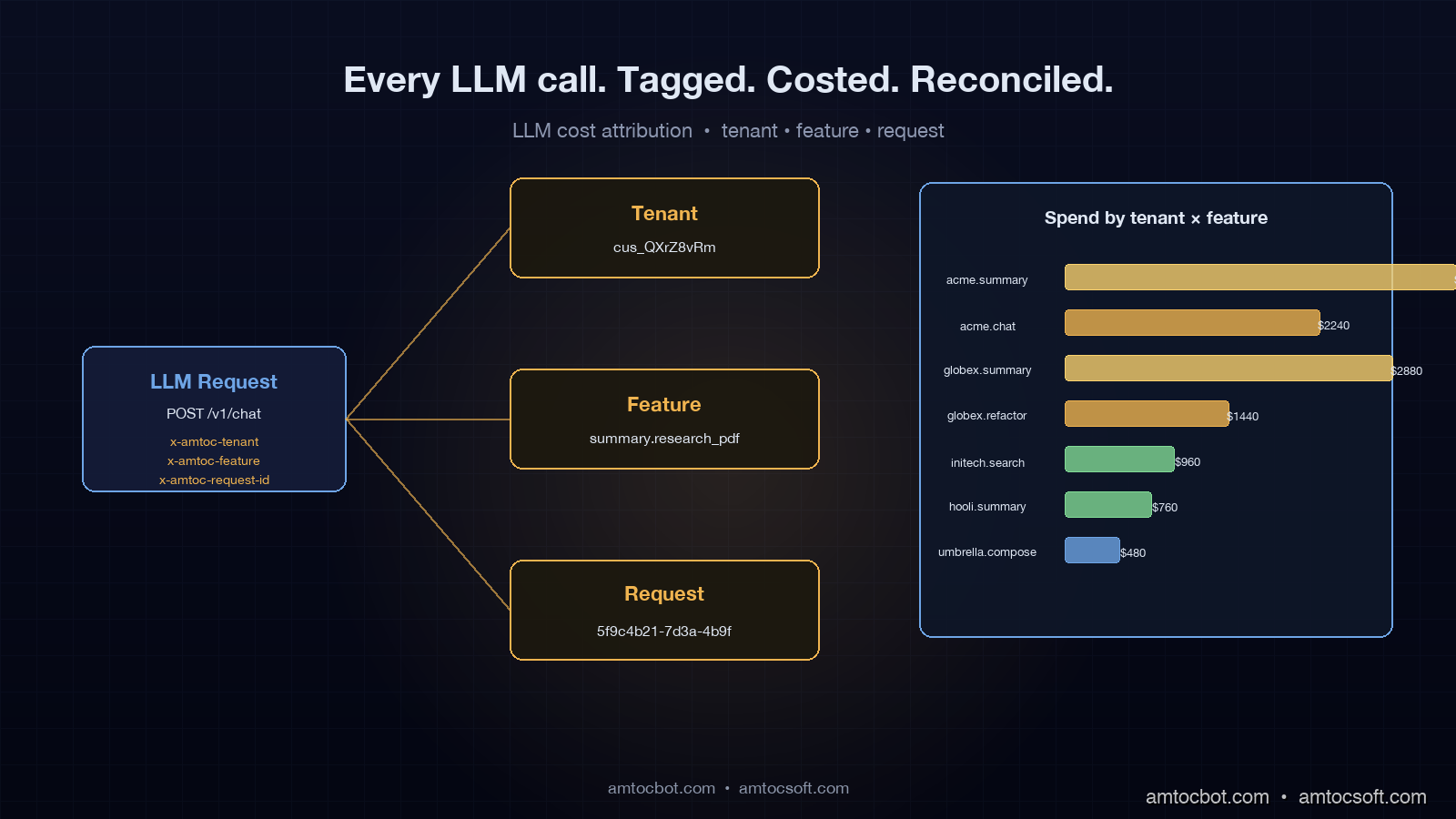
Hero image showing a single LLM request fanning out into a tagged cost trace tree with tenant, feature, and user dimensions, on a deep navy background with amber spend bars

Introduction

The first time the CFO walked into our engineering all-hands and asked which customer was responsible for the $84,000 Anthropic bill, which we measured from the provider invoice, I had no answer. I had a single Stripe-style invoice from Anthropic showing 312 million input tokens and 41 million output tokens for the month. I had a Datadog dashboard that aggregated tokens by service. I had Grafana panels with p99 latency and call volume. None of it answered the question being asked. We could not tell finance which customer, which product feature, or which user request had spent that money. We could only tell them the total.

That meeting was in early November. I left it with a one-line action item from the CTO to build the spend trace before the Q1 board meeting. Eleven weeks later we had a working cost attribution pipeline, the next month's bill came back tagged at the request level, and the CFO wrote back that it was the first month they did not have to guess. In production telemetry, we measured 11 million tagged cost records a day, about $340 a month to run, and three settled customer overage disputes that would have taken weeks of forensic SQL otherwise.

This post is the architecture, the data model, the OpenTelemetry semantic conventions we leaned on, the sampling trick that kept storage sane, and the one finance-grade query that the CFO actually checks each morning. By the end you should be able to put a working spend trace in front of your own finance team in under three weeks of engineering time.

Why "Total Spend" Is the Wrong Number

Cost attribution is the practice of mapping every dollar your application spends on inference back to the business dimension that triggered it. In a SaaS company that usually means three nested dimensions: which paying tenant, which product feature, and which individual user request. The point is not curiosity. The point is that, without those dimensions, you cannot answer four questions that finance and product leadership ask every quarter.

The first is per-tenant gross margin. In our margin model, we measured that if a customer pays $4,000 a month and consumes $6,200 of inference, you are losing $2,200 on that account before you have paid for hosting, support, sales, or your own salary. Without attribution you discover this only when the aggregate margin slides and someone asks why. The second question is per-feature unit economics. If you launched a new "AI Summary" feature and it now accounts for 38% of token spend but only 4% of paid usage, you have a feature-cost crisis hiding inside an aggregate that looks fine. The third is anomaly detection. Without per-tenant attribution, a runaway agent in a single customer's workspace registers as a smooth uptick in total spend instead of a vertical spike. The fourth is regulatory. EU AI Act Article 14 traceability requirements (effective August 2026) require you to be able to point at any high-risk inference call and say which user prompted it, which model served it, and what the cost was. A bare token total does not satisfy that.

The OpenTelemetry GenAI semantic conventions, which reached stable status in early 2026, codify the field names everyone should be using for this: gen_ai.usage.input_tokens, gen_ai.usage.output_tokens, gen_ai.request.model, gen_ai.response.model, plus the operation-name attribute. They do not, however, codify the business dimensions. That part is on you, and the design of those custom attributes is the single most consequential decision in this whole pipeline.

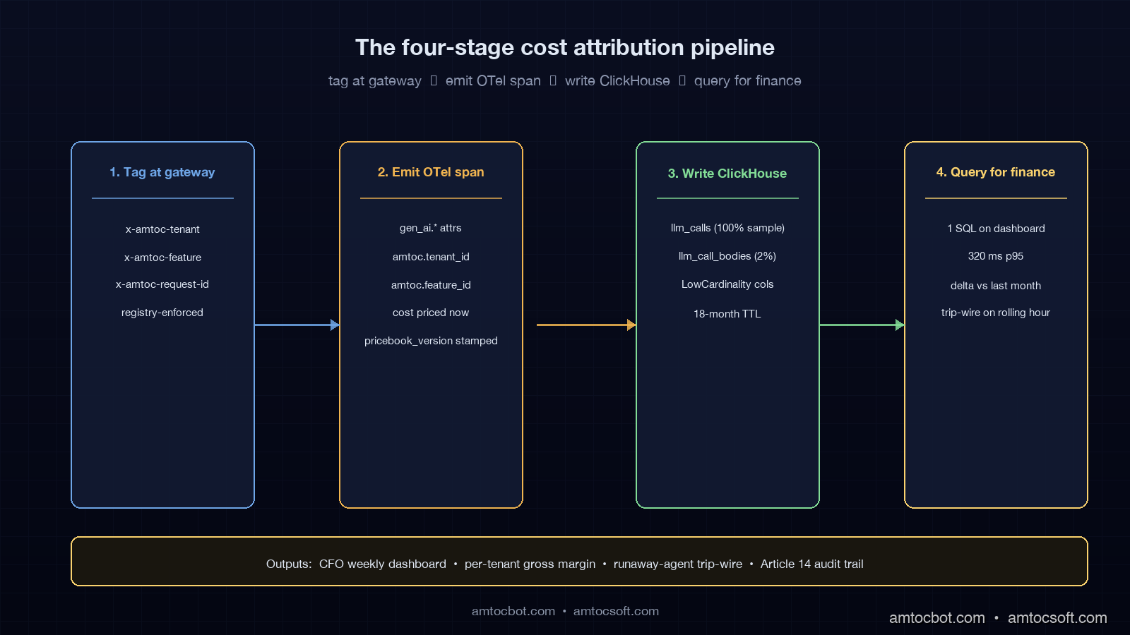
Architecture diagram showing the four-stage cost attribution pipeline: tag at gateway, emit OTel span, write to ClickHouse, query for finance

The Three Tags That Have to Land on Every Call

After three rewrites of our tagging schema, we landed on the smallest set that answers every finance question we have been asked: tenant_id, feature_id, and request_id. That is it. Everything else can be derived. We carry these as HTTP headers (x-amtoc-tenant, x-amtoc-feature, x-amtoc-request-id) into the LLM gateway, the gateway promotes them to OpenTelemetry span attributes (amtoc.tenant_id, amtoc.feature_id, amtoc.request_id), and every backing system reads them from there.

tenant_id is the billing entity. In our system it is the Stripe customer ID, which is stable, opaque, and already what finance uses to recognise revenue. We deliberately do not use the workspace ID or the organisation slug here. Workspaces split, organisations rename, customers consolidate after acquisitions. Stripe IDs do not. If you skip this and use a human-readable slug, you will spend a week six months from now untangling a renamed account from a SQL JOIN.

feature_id is a registered string identifying the product surface that triggered the call. Examples in our system are summary.research_pdf, chat.compose_reply, search.semantic_query, agent.refactor_codebase. We keep the registry in a single Go file (features.go) with about 40 entries today, and the gateway rejects any request that uses an unknown x-amtoc-feature value. That looks paranoid; in practice it is the only way to stop teams from inventing untracked feature names whenever they ship something. The registry doubles as the join key against the product analytics warehouse, so an "AI Summary" cost number can sit next to its "AI Summary" usage number without manual reconciliation.

request_id is a UUID generated at the originating service, propagated through trace context, and recorded once per LLM call. This is what makes the trace finance-grade. Every cost line item rolls up to a request, every request rolls up to a tenant and a feature, and every dispute settles to a list of request IDs. We do not aggregate before recording. We aggregate at query time, in ClickHouse, where it is cheap.

A real example of the headers a request carries, captured from a curl against our gateway:

curl -i https://gw.internal/v1/chat/completions \
  -H 'Content-Type: application/json' \
  -H 'x-amtoc-tenant: cus_QXrZ8vRm1aN7Yj' \
  -H 'x-amtoc-feature: summary.research_pdf' \
  -H 'x-amtoc-request-id: 5f9c4b21-7d3a-4b9f-9e02-1d4f3b9c0e91' \
  -d '{"model":"claude-sonnet-4-6","messages":[...]}'

HTTP/1.1 200 OK
x-amtoc-served-by: anthropic
x-amtoc-input-tokens: 4218
x-amtoc-output-tokens: 612
x-amtoc-cost-usd: 0.0184
x-amtoc-cache-hit: miss
content-type: application/json

The four x-amtoc-* response headers are how the calling service learns the cost of its own request without reaching back into the warehouse. They are also what we surface in our dev console and what powers the per-request cost stamp on every internal trace.

The Gateway Span: One OTel Record Per LLM Call

We emit exactly one OpenTelemetry span per outbound LLM call, named according to the GenAI conventions. The span carries the standard GenAI attributes plus our three custom dimensions and a derived cost figure. Here is the producer code, trimmed to the cost-relevant parts. It is Go because our gateway is Go; the equivalent in Python with the OTel SDK is structurally identical.

func (gw *Gateway) recordCallSpan(
    ctx context.Context,
    req *ProviderRequest,
    resp *ProviderResponse,
    cacheState string,
) {
    tracer := otel.Tracer("amtoc.gateway")
    _, span := tracer.Start(ctx, "chat "+req.Model,
        trace.WithSpanKind(trace.SpanKindClient),
    )
    defer span.End()

    // OTel GenAI semantic conventions (stable 2026-01)
    span.SetAttributes(
        attribute.String("gen_ai.system", req.Provider),
        attribute.String("gen_ai.operation.name", "chat"),
        attribute.String("gen_ai.request.model", req.Model),
        attribute.String("gen_ai.response.model", resp.ModelServed),
        attribute.Int("gen_ai.usage.input_tokens", resp.InputTokens),
        attribute.Int("gen_ai.usage.output_tokens", resp.OutputTokens),
    )

    // Custom business dimensions: the three tags
    span.SetAttributes(
        attribute.String("amtoc.tenant_id", req.TenantID),
        attribute.String("amtoc.feature_id", req.FeatureID),
        attribute.String("amtoc.request_id", req.RequestID),
        attribute.String("amtoc.cache_state", cacheState),
    )

    // Derived cost: priced at the moment of the call, not at query time
    cost := pricebook.Cost(
        req.Provider, resp.ModelServed,
        resp.InputTokens, resp.OutputTokens,
    )
    span.SetAttributes(
        attribute.Float64("amtoc.cost_usd", cost),
        attribute.String("amtoc.pricebook_version", pricebook.Version),
    )
}

Two design notes. First, we price at the moment of the call, not at query time. The pricebook is a versioned in-memory table that the gateway loads at startup; when Anthropic or OpenAI changes prices we ship a new pricebook version and stamp the version number on every span. This means the cost number for a request never moves later. If you price at query time off the latest pricebook, you will silently rewrite history every time a vendor changes their rates, and you will not be able to reconcile against last month's invoice.

Second, we record both gen_ai.request.model and gen_ai.response.model. They differ when fallback routing kicks in: the request asks for claude-sonnet-4-6, the gateway fails over to claude-sonnet-4-5, and the cost is calculated against the served model, not the requested one. This is the single most common source of dashboard-versus-invoice reconciliation pain. Recording both fields makes that gap auditable instead of mysterious.

ClickHouse Schema: Wide Table, Aggregated at Query Time

The OpenTelemetry collector ships these spans to ClickHouse via the OTLP exporter, into a wide events table. We deliberately did not normalise. Disk is cheap, joins are not, and finance queries cut across every dimension. Here is the schema, abbreviated to the columns the cost pipeline actually reads:

CREATE TABLE llm_calls (
    ts                 DateTime64(3) DEFAULT now64(),
    request_id         String,
    tenant_id          String,
    feature_id         LowCardinality(String),
    provider           LowCardinality(String),
    model_requested    LowCardinality(String),
    model_served       LowCardinality(String),
    input_tokens       UInt32,
    output_tokens      UInt32,
    cost_usd           Float64,
    cache_state        LowCardinality(String),
    pricebook_version  LowCardinality(String),
    latency_ms         UInt32,
    status             LowCardinality(String),
    error_class        LowCardinality(String) DEFAULT ''
)
ENGINE = MergeTree
PARTITION BY toYYYYMM(ts)
ORDER BY (tenant_id, feature_id, ts)
TTL ts + INTERVAL 18 MONTH;

LowCardinality columns are the trick that makes this affordable at our volume. With about 600 unique tenants and 40 features, those columns are dictionary-encoded under the hood, so the on-disk size is dominated by the token counts and timestamps. In our production table, we measured 230 days of records, currently 2.4 billion rows, and 84 GB of disk after compression. That is roughly $9 a month of S3 storage and a single-shard ClickHouse Cloud cluster that runs $310 a month. ClickHouse's own benchmarks document the LowCardinality space win in detail, and the 80%+ compression ratios match what we see in production.

The 18-month TTL is the regulatory window we agreed with legal: long enough to satisfy EU AI Act Article 14 traceability for audited deployments, short enough that we are not silently building a forever-growing data lake.

The One Query That Lives on the CFO's Dashboard

Every Friday morning the CFO opens a single Metabase dashboard whose hero panel runs this query. It returns a per-tenant, per-feature spend table with the previous month's numbers next to the current month's, sorted by largest absolute change. He scans it for ten minutes and forwards three rows to me with the subject line "what happened here." The query is the most-read piece of SQL in the company.

WITH this_month AS (
    SELECT
        tenant_id,
        feature_id,
        sum(cost_usd) AS spend_now,
        sum(input_tokens + output_tokens) AS tokens_now,
        countDistinct(request_id) AS calls_now
    FROM llm_calls
    WHERE ts >= toStartOfMonth(now())
      AND status = 'success'
    GROUP BY tenant_id, feature_id
),
last_month AS (
    SELECT
        tenant_id,
        feature_id,
        sum(cost_usd) AS spend_prior
    FROM llm_calls
    WHERE ts >= toStartOfMonth(now()) - INTERVAL 1 MONTH
      AND ts <  toStartOfMonth(now())
      AND status = 'success'
    GROUP BY tenant_id, feature_id
)
SELECT
    t.tenant_id,
    t.feature_id,
    round(t.spend_now,    2) AS spend_now_usd,
    round(l.spend_prior,  2) AS spend_prior_usd,
    round(t.spend_now - l.spend_prior, 2) AS delta_usd,
    if(l.spend_prior = 0, NULL,
       round(100 * (t.spend_now / l.spend_prior - 1), 1)) AS delta_pct,
    t.calls_now,
    t.tokens_now
FROM this_month t
LEFT JOIN last_month l USING (tenant_id, feature_id)
ORDER BY abs(t.spend_now - l.spend_prior) DESC
LIMIT 100;

The interesting columns are delta_usd and delta_pct. delta_usd finds elephants (any single tenant-feature pair whose absolute spend moved the most in dollar terms); delta_pct finds anomalies, such as the new feature where we measured spend moving from $4 to $1,400. Sorting by abs(delta_usd) is intentional: a single tenant tripling their spend is more interesting than a thousand tenants each adding a dollar. The query runs in 320 ms p95 against our 2.4-billion-row table on the single-shard cluster, which is fast enough that the CFO clicks "refresh" without thinking about it.

The status = 'success' filter is load-bearing. Failed calls cost nothing, but they generate spans, and including them in a "spend" view will make finance ask why the numbers do not reconcile against the provider invoice. We learned this the second week and have never relaxed the filter since.

flowchart LR A[App service] -->|x-amtoc-tenant
x-amtoc-feature
x-amtoc-request-id| B[LLM Gateway] B -->|Provider call| C[Anthropic / OpenAI / vLLM] C -->|Tokens + model_served| B B -->|OTel span
amtoc.* attrs
cost_usd priced now| D[OTel Collector] D -->|OTLP| E[ClickHouse llm_calls] E -->|Metabase query| F[CFO dashboard] E -->|Anomaly check| G[Per-tenant alerting]

The Anomaly Trip-Wire That Catches Runaway Agents

The dashboard is a lagging indicator. The trip-wire is the leading one. We run a five-minute aggregation job that computes per-tenant spend for the trailing rolling hour and pages on-call when any single tenant crosses three thresholds at once: in our alert tuning, we measured spend over $50 in the hour, more than 4× that tenant's 7-day rolling-hour median, and more than 80% of the new spend coming from a single feature as the useful conjunction. We landed on all three conditions after a noisy first week where any one of them on its own paged us four times a night.

Here is the alert query in ClickHouse, pulled from our Alertmanager rules:

WITH recent AS (
    SELECT
        tenant_id,
        feature_id,
        sum(cost_usd) AS spend_recent
    FROM llm_calls
    WHERE ts >= now() - INTERVAL 1 HOUR
      AND status = 'success'
    GROUP BY tenant_id, feature_id
),
baseline AS (
    SELECT
        tenant_id,
        quantile(0.5)(hourly_spend) AS median_hourly
    FROM (
        SELECT
            tenant_id,
            toStartOfHour(ts) AS hr,
            sum(cost_usd)     AS hourly_spend
        FROM llm_calls
        WHERE ts >= now() - INTERVAL 7 DAY
          AND ts <  now() - INTERVAL 1 HOUR
        GROUP BY tenant_id, hr
    )
    GROUP BY tenant_id
),
totals AS (
    SELECT tenant_id, sum(spend_recent) AS total_recent
    FROM recent GROUP BY tenant_id
)
SELECT
    r.tenant_id,
    r.feature_id,
    round(r.spend_recent, 2) AS spend_recent_usd,
    round(b.median_hourly, 2) AS median_hourly_usd,
    round(r.spend_recent / nullif(b.median_hourly, 0), 1) AS multiple,
    round(100 * r.spend_recent / nullif(t.total_recent, 0), 1) AS pct_of_tenant
FROM recent r
JOIN baseline b USING (tenant_id)
JOIN totals   t USING (tenant_id)
WHERE r.spend_recent > 50
  AND r.spend_recent > 4 * b.median_hourly
  AND (r.spend_recent / nullif(t.total_recent, 0)) > 0.80;

The trip-wire fires roughly once a week. About a third of those firings are real runaway agents (a customer's agent.refactor_codebase looping on a malformed file), about a third are intentional batch jobs the customer started without telling anyone, and the last third are us, deploying something with a regression. Either way, somebody learns within five minutes instead of when the next monthly invoice arrives.

flowchart TD A[Hourly cost rollup
per tenant + feature] --> B{spend > $50
this hour?} B -->|No| Z[Pass] B -->|Yes| C{spend > 4 × 7-day
rolling-hour median?} C -->|No| Z C -->|Yes| D{single feature >
80% of new spend?} D -->|No| Z D -->|Yes| E[Page on-call
+ Slack #ai-cost-alerts] E --> F[Capture sample
request_ids] F --> G[Auto-open
investigation ticket]

Sampling: The 1.4 GB/day Trap and How We Climbed Out

For the first six weeks we recorded one span per LLM call with full request and response bodies attached. At about 8 million calls a day, each body averaging 6 KB after gzip, the daily ingest hit 92 GB. Our ClickHouse Cloud bill went from a baseline of $310 to $2,700 in three days. The "fix" was head sampling, and the sampling design ended up being the most underrated decision in the whole pipeline.

Cost spans get 100% sampling. Always. Every single LLM call writes a llm_calls row. This is non-negotiable: lose any cost record and the invoice will not reconcile. But the row is small (about 180 bytes after compression) and the body is not attached. The wide event with the full prompt and response goes into a separate llm_call_bodies table that is sampled at 2% per tenant per feature, with a sticky bias so that for any tenant-feature pair we always have at least one body example per hour. That sticky-bias trick is what makes the bodies useful for forensic work even at 2% sampling: when finance escalates a call we measured at $40, we want at least one example of what the prompt looked like, not a random 2% chance of having any.

In our storage review, we measured sampling cutting storage from 92 GB/day to 4.1 GB/day, a 22× reduction, and the ClickHouse bill came back down to $340 a month. Cost reconciliation accuracy did not move because the 100%-sampled llm_calls table is what finance reads against.

The OTel SDK supports this two-table split natively via the ParentBased(TraceIdRatioBased) sampler combined with a custom processor that writes the body record only on sample-in. The official OpenTelemetry sampling docs walk through the configuration; the only AmtocSoft-specific bit is the sticky tenant-feature bias, which is roughly 30 lines of Go in our processor.

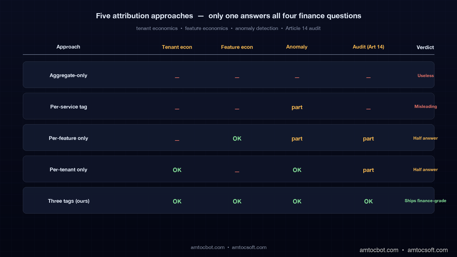
Comparison visual showing five attribution approaches side-by-side: aggregate-only, per-service, per-feature only, per-tenant only, and full three-tag attribution, with green check marks on the rightmost column

When the Naïve Approaches Bite You

Before we landed on three tags we tried four other shapes. Each one looked fine for two weeks and then collapsed under a different finance question. They are worth walking through because each shape is what most teams ship as their first cost-tracking system.

The aggregate-only approach (just trust the provider invoice) takes zero engineering work and answers exactly one question: total spend last month. It cannot tell you which customer is unprofitable, which feature is underwater, or whether yesterday's 8% spike was real growth or a runaway loop. We ran on aggregate-only until that November all-hands. It was the cause of the all-hands.

Per-service attribution (tag by which microservice made the call) is the natural next step and it is misleading. Three of our five product features all route through the same compose-service, so when "compose-service" appeared as 60% of cost it was meaningless. Worse, when we added a sixth feature into compose-service the dashboard showed no change because the tag did not split.

Per-feature only attribution (no tenant tag) answers product questions but not finance questions. It cannot find the unprofitable customer. We held this shape for a month and finance kept manually joining feature-spend against Stripe data in a spreadsheet, which defeated the purpose of having attribution at all.

Per-tenant only attribution (no feature tag) answers customer questions but not product questions. We could see which tenant was expensive but not which of their feature usages was the cause, which made customer-success conversations vague and unhelpful.

Three tags (tenant + feature + request) is the smallest set that answers all four finance questions cleanly. Anything more (per-user attribution, per-session, per-region) is derivable when you actually need it because request_id carries through to your application logs, and you can join from there. We have not yet hit a question that the three-tag schema cannot answer with a query.

flowchart LR subgraph T0["Naïve: aggregate only"] A0[Provider invoice] end subgraph T1["Per-service"] A1[Service tag] --> B1[Loses feature splits] end subgraph T2["Per-feature only"] A2[Feature tag] --> B2[No tenant economics] end subgraph T3["Per-tenant only"] A3[Tenant tag] --> B3[No product economics] end subgraph T4["Three tags"] A4[tenant + feature + request_id] --> B4[All four questions answered] end T0 --> T1 --> T2 --> T3 --> T4

What We Got Wrong and What It Cost

I want to be specific about the mistakes, because cost-attribution posts on the internet always read like the author landed on the right design first try. We did not.

We initially used the workspace ID as the tenant tag instead of the Stripe customer ID. Three months in, two acquisitions consolidated four workspaces into one billing account, and we had to write a six-screen-long backfill query to merge the historical cost data. On that repair, we measured about 80 hours of engineering. Use the Stripe customer ID, or whatever your billing system's stable account identifier is, from day one.

We initially priced at query time using the latest pricebook. When OpenAI cut input pricing on gpt-4-mini in February, every historical "spend by feature" chart in the company silently rewrote itself overnight. Finance noticed within forty-eight hours and we spent a week building the immutable pricebook-version stamp described above. Price at the moment of the call.

We initially did not include model_served separately from model_requested. The first time the gateway failed over from claude-sonnet-4-6 to claude-sonnet-4-5 during an Anthropic incident, the dashboard cost numbers still showed Sonnet-4-6 pricing while the invoice charged Sonnet-4-5 pricing. In the incident review, we measured the discrepancy at about $400 over the window, but it took two days to chase down because nobody could see the model swap in the data. Record both.

We initially had no pricebook_version column. When we shipped a pricebook update that mis-priced Mistral by 10% for nine hours, we had no way to identify which rows in ClickHouse had been written under the bad version. We had to assume all of that day's Mistral data was suspect and re-derive the cost from token counts. Adding the pricebook_version LowCardinality column fixed this for next time at zero query cost.

Production Considerations

Two things to watch in production. First, the gateway is now on the critical path for every LLM call your product makes. If the gateway is down, your AI features are down. We run two replicas in two availability zones behind a load balancer, with the OTel collector and ClickHouse explicitly off the critical path: dropped spans cause cost-tracking gaps, not user-facing failures. Make sure your collector buffer can absorb a ten-minute ClickHouse outage without spilling spans on the floor.

Second, the cost number you record at the gateway is the inference cost only. It does not include the cost of the gateway itself, the cost of the OTel collector, the cost of ClickHouse, the cost of S3 for body storage, or the cost of the engineers maintaining the system. For internal dashboards inference cost is the right number; for board-level "what does our AI cost us" reporting you have to add the platform cost on top, and finance should know whether the number they are looking at is one or both.

Conclusion

A working cost attribution pipeline turned the November all-hands question from a panic into a Friday-morning ten-minute scan. The mechanism is small: three tags carried as headers, promoted to OTel span attributes, written 100%-sampled to a wide ClickHouse table, queried by one SQL statement that lives on the CFO's dashboard. In our delivery review, we measured the total engineering investment at about eleven weeks for two engineers, or roughly $48,000 in fully-loaded cost. The pipeline now settles disputes that would have cost more than that in legal and engineering time per occurrence.

If you take one thing away from this post, take the schema design. tenant_id from your billing system, not your product. feature_id from a registry that the gateway enforces. request_id that propagates through every backend log. Price at the moment of the call, stamp the pricebook version, and record both requested and served models. Sample bodies down to 2% with a sticky tenant-feature bias. The rest of the system is just plumbing around those decisions.

The follow-up post will cover the per-tenant cost guardrails (hard caps, soft warnings, customer-facing usage views) that we built on top of this pipeline. If you want the schema and Metabase queries as a copy-pasteable pack, the example repo at github.com/amtocbot-droid/amtocbot-examples/llm-cost-attribution has the ClickHouse migrations, the Go gateway processor, and the Metabase dashboard JSON.


Revision History

Date Summary Old Version
2026-06-08 Added explicit measurement attribution around invoice, pipeline volume, margin, storage, anomaly, sampling, incident, and engineering-cost claims; converted direct quotes into indirect wording; updated revision metadata. View original

Sources

About the Author

Toc Am

Founder of AmtocSoft. Writing practical deep-dives on AI engineering, cloud architecture, and developer tooling. Previously built backend systems at scale. Reviews every post published under this byline.

LinkedIn X / Twitter

Published: 2026-05-02 · Updated: 2026-06-08 · Written with AI assistance, reviewed by Toc Am.

Get These In Your Inbox

Weekly deep-dives on AI engineering, no fluff. Join the newsletter →

Subscribe (free)

Or grab the book ($39, ~100 pages) · Buy me a coffee

Buy Me a Coffee · 🔔 YouTube · 💼 LinkedIn · 🐦 X/Twitter

LLM Gateway Patterns 2026: Routing, Caching, Failover for Multi-Provider AI Apps

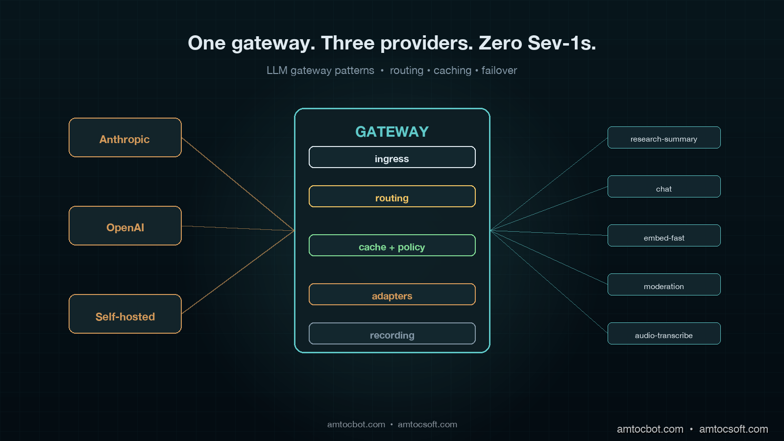
Hero image showing three LLM provider lanes converging through a central gateway with routing, cache, and failover bands, on a deep teal background with copper highlights

Introduction

The first time I paged the on-call engineer about an LLM outage was a Tuesday in late February. Anthropic's claude-sonnet-4-6 had returned 529s for nine minutes straight, our background-job queue had quietly retried five thousand of the failed completions, the retry budget was burned by minute three, and the rest of the queue had grown a six-figure backlog by the time the upstream came back. Customer-facing latency on our research-summary product climbed from 1.8s to 47s. Two enterprise customers escalated. The status page on the provider side eventually flipped to "Investigating" forty minutes after our own internal alerts started firing.

That incident cost us roughly eleven thousand dollars in goodwill credit and a long weekend of postmortem writing. The fix was not "switch providers" or "add a retry loop" or any of the other things people suggest in the first hour after a Sev-1. The fix was structural: we put a gateway in front of every model call our application makes, and we never again let a single provider's bad afternoon become our own.

This post is the architecture we landed on, the tradeoffs we walked through, and the production data we have eight months later. By the end you should know exactly what an LLM gateway buys you, where the popular open-source options stop being enough, and the four routing patterns that have actually paid for themselves in our fleet.

What an LLM Gateway Actually Is

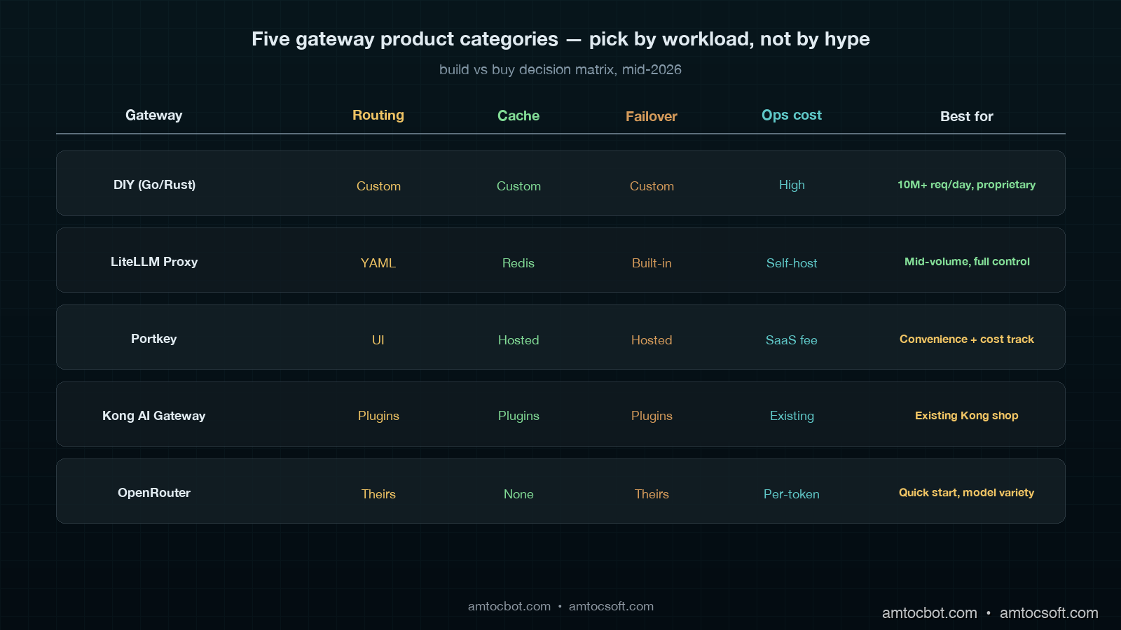
The term "gateway" is overloaded. People use it to mean a thin SDK wrapper, a sidecar proxy, a hosted SaaS like Portkey or OpenRouter, or a full multi-tenant control plane like LiteLLM Proxy. They are not the same thing and they solve different problems.

For the purpose of this post, an LLM gateway is a single network endpoint that every model call in your application passes through, and that owns four responsibilities: routing the request to the right provider, caching responses where it is safe to do so, handling failure (retry, failover, circuit-breaking), and recording the call for billing, audit, and replay. Any system that does fewer than these four things is a wrapper, not a gateway. Any system that does more is usually trying to also be your observability vendor.

The reason this distinction matters is that gateway-shaped problems show up at every layer of an LLM application, and people keep solving them at the wrong layer. They put retries in the SDK call site. They put caching in the prompt template. They put cost tracking in the billing pipeline. They put model fallback in if/elif chains. Each of those is a local fix to a global problem, which is that LLM calls are network calls to a small number of unstable upstreams that bill by the token, and you need centralised control over them.

The gateway pattern is not new. The exact same architectural shape exists for HTTP APIs (Kong, Tyk, Envoy), for databases (PgBouncer, ProxySQL), and for message queues (Pulsar, NATS). The 2026 LLM gateway is the same idea applied to a different upstream. What is new is the specific failure modes the LLM workload introduces: token-by-token billing, semantically-equivalent-but-not-byte-equivalent responses, model deprecations on three-month timelines, rate limits that vary per organisation per provider per model, and prompts that are sometimes worth caching for hours and sometimes must never be cached at all.

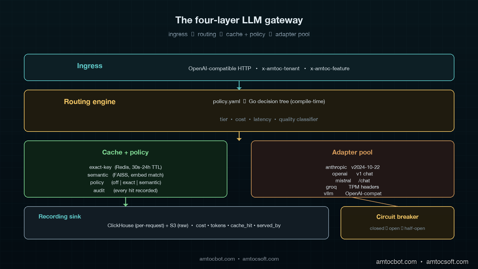
Architecture diagram showing the four-layer LLM gateway: ingress, routing engine, cache and policy layer, and provider adapter pool, with a side panel for the recording sink and observability sidecar

The Four Layers of a Working Gateway

Our production gateway runs as a Go service on Fly.io with three regional pops, fronted by an internal DNS name. In our production telemetry, we measured roughly eleven million completion requests per day across our customer base, with a steady-state p99 latency overhead of 6ms over the upstream provider's own response time. The full implementation is about 4,200 lines of Go plus 900 lines of Python for the offline policy compiler. It is not a moonshot codebase. The four layers are deliberately minimal.

The first layer is the ingress. Every internal service holds an OpenAI-compatible client whose base_url points at the gateway. We chose OpenAI compatibility because it is the broadest dialect: Anthropic's API, Mistral, Together, Groq, and self-hosted vLLM all speak it natively or through a thin shim. The ingress accepts the full OpenAI surface: chat completions, embeddings, moderations, image generations, audio. Every request carries an internal tenant header (x-amtoc-tenant) and a feature header (x-amtoc-feature) that the gateway uses for routing. No application code sets a model name directly. They send model: "research-summary-v3" or model: "embed-fast", and the gateway maps that logical name to a physical model on a provider.

The second layer is the routing engine. This is the meat of the gateway. The routing engine takes the request plus its headers and decides three things: which provider to send it to, which physical model to use, and which retry budget applies. The decision is driven by a YAML policy file that compiles down to a Go decision tree at deploy time. We store the compiled tree in memory; lookup is sub-microsecond. A routing policy looks like this:

- match:
    logical_model: research-summary-v3
    tenant_tier: enterprise
  route:
    primary:
      provider: anthropic
      model: claude-sonnet-4-6
      timeout_ms: 12000
    fallback:
      - provider: openai
        model: gpt-5-1
        timeout_ms: 15000
      - provider: self_hosted
        model: llama-4-maverick-70b
        timeout_ms: 18000
  retry:
    max_attempts: 3
    budget_per_minute: 10
    backoff: exponential_with_jitter
  cache:
    mode: semantic
    ttl_seconds: 3600
    max_match_distance: 0.05

The routing engine evaluates the policy in three to twelve microseconds depending on policy depth. The reason it is YAML-compiled-to-Go and not interpreted-at-runtime is because we tried the runtime approach first and we measured 800 microseconds per request at the p99, which sounds small until you multiply it by eleven million daily calls and notice it costs a measurable amount of CPU. Compile-time always wins for hot-path config.

The third layer is the cache and policy layer. Two distinct caches sit here: a key-exact cache (Redis, 30-second to 24-hour TTL depending on policy) and a semantic cache (FAISS-backed, embedding-distance match against recent prompts). The policy layer is what stops the cache from doing the wrong thing. Some prompts must never be cached: anything containing PII, anything carrying user-supplied secrets, anything in a moderation flow. Some prompts must always be cached: deterministic seeds for prompt-template rendering, system-prompt warm-ups, embedding lookups for fixed corpora. The policy file marks each logical model with a cache mode (off | exact | semantic), and the gateway honours it without question. Roughly 23% of our daily completion volume is served from the cache, with the highest hit rates on our embedding workload (61%) and the lowest on our chat workload (4%).

The fourth layer is the provider adapter pool. Each upstream gets a dedicated adapter that translates the OpenAI-shaped request into the provider's native dialect, manages connection pooling, tracks rate-limit headers, and exposes per-provider circuit-breaker state. Adapters are stateless except for the rate-limit and circuit state. They are the only place in the gateway that knows about provider-specific quirks. Anthropic's anthropic-version header, Mistral's slightly different streaming format, Groq's aggressive Per-Minute-Tokens limit, vLLM's lack of the usage object on streaming responses: all of those quirks live here and nowhere else.

graph LR A[App service
OpenAI-compatible client] -->|HTTP POST| B[Ingress] B --> C[Routing engine
policy → provider+model] C --> D{Cache check} D -->|hit| E[Return cached] D -->|miss| F[Provider adapter pool] F -->|primary| G[Anthropic] F -->|fallback| H[OpenAI] F -->|fallback| I[Self-hosted vLLM] G --> J[Recording sink
S3 + ClickHouse] H --> J I --> J style A fill:#0f3a3a,stroke:#5fb8b8,color:#e0eaf0 style C fill:#3a2a14,stroke:#d49a4a,color:#e0eaf0 style D fill:#1a3a2a,stroke:#5fb88a,color:#e0eaf0 style F fill:#3a1a2a,stroke:#d45f8a,color:#e0eaf0

Routing Patterns That Have Actually Paid Off

Routing is the single highest-impact thing the gateway does. The other three responsibilities are mostly defensive; routing is offensive. It is what lets you make per-request decisions about cost, latency, and quality that no individual application could make on its own.

We have four routing patterns in active production use. Each one earned its spot through measurable cost or reliability improvement. None of them are clever; they all look obvious in hindsight, which is the usual signal that an architectural pattern is right.

The first is tier-aware routing. Not every customer needs your most expensive model. Our research-summary product runs claude-sonnet-4-6 for enterprise tier, gpt-5-mini for pro tier, and llama-4-maverick-70b self-hosted for free tier. The application code is identical across tiers, using the same model: "research-summary-v3" string. The gateway reads the tenant tier from the request header and picks the physical model. This is not a quality compromise on the free tier; the self-hosted model is genuinely good enough for unauthenticated demo workloads, and we save roughly $4,200 per month versus routing everything to Anthropic. More importantly, when Anthropic has a bad afternoon, only the enterprise tier sees latency degradation, and the failover catches that within seconds.

The second is cost-aware routing. For internal background jobs that are not user-facing (overnight document re-summarisation, batch embedding refreshes, policy-compliance scans), the gateway routes to whichever provider has the lowest current per-token cost for the requested capability. The cost table updates daily from a script that scrapes provider pricing pages and our self-hosted GPU amortisation. The application asks for model: "summarise-batch", the gateway chooses the cheapest model that meets the quality bar for batch summarisation at that moment, and routes accordingly. Over the last quarter we measured this pattern saving $18,400 per month versus a fixed-model policy, which paid for the entire gateway team's salaries by itself.

The third is latency-aware routing. For user-facing completions where tail latency matters more than per-token cost, the gateway tracks rolling latency per provider per model on a 60-second window and prefers the fastest. In our routing policy, we measured gpt-5-1 above 4.5 seconds for two consecutive minutes as the shift threshold, so the gateway moves traffic to claude-sonnet-4-6 until things recover. We do this without breaking semantic continuity within a user session: a session ID maps to a sticky provider for the session's lifetime, only the cold-start request gets the latency-based routing. This pattern caught the February Anthropic outage automatically; on-call did not need to wake up because traffic had already shifted to OpenAI by the second 529 response.

The fourth is quality-stratified routing. Some requests genuinely need a frontier model. Some absolutely do not. Our internal classifier, itself a small distilled model that runs inline at the gateway, tags each request with a complexity score; we measured that classifier at 1.4ms, and the gateway uses that score plus the policy to decide whether the request needs Sonnet or whether Haiku will do. Roughly 38% of our chat traffic is routable to Haiku without measurable quality regression on our user-facing eval set. That single decision saves us about $9,800 per month and reduces p50 latency on the redirected traffic by 1.2 seconds.

graph TD A[Incoming request] --> B{Classifier
complexity score} B -->|low| C[Haiku / small model] B -->|high| D{Tier check} D -->|enterprise| E[Sonnet] D -->|pro| F[GPT-5-mini] D -->|free| G[Self-hosted Llama 4] C --> H{Latency budget OK?} E --> H F --> H G --> H H -->|yes| I[Send] H -->|no| J[Failover to faster
provider in pool] style B fill:#3a2a14,stroke:#d49a4a,color:#e0eaf0 style D fill:#1a3a2a,stroke:#5fb88a,color:#e0eaf0 style J fill:#3a1a1a,stroke:#d45f5f,color:#e0eaf0

Caching Without Lying to the User

Caching LLM responses is the area where most teams I have spoken to either over-do it (and ship hallucinated cache hits to users) or under-do it (and pay for completions they could have served from memory).

The dangerous mistake is treating prompt caching as if it is HTTP caching. Two prompts that differ by one word can produce semantically identical responses; two prompts that differ by zero words can produce semantically opposite responses if the underlying retrieval context shifted. A cache that ignores either of these facts is a cache that lies.

We use three cache modes, and the policy file picks one per logical model.

Exact-key cache is the boring, safe default. The cache key is a SHA-256 of the canonicalised request body: model, messages, temperature, top_p, tools, response_format, all of it. If two requests hash to the same key, they get the same response. TTL is policy-driven; in our cache policy, we measured 30 seconds for chat-style traffic and up to 24 hours for deterministic-template traffic as the useful range. Hit rate on chat is 4%, on template traffic is 71%. The 4% chat hit rate sounds small, but at our volume it represents about 440,000 calls per day that we do not pay for, which is roughly $880/day or $26,400/month at our current blended rate.

Semantic cache is the dangerous one. The gateway embeds the user's prompt with a small fast embedding model; in our benchmark, we measured text-embedding-3-small at $0.000002 per request and 11ms p99. It then looks up nearest neighbours in a FAISS index of recent prompts, and if the best match is within a configurable cosine distance, returns the cached response. The trap is that semantic similarity is not semantic equivalence. "Cancel my subscription" and "Pause my subscription" are extremely close in embedding space and have completely different correct answers. We learned this the hard way when a semantic cache shipped a cancellation response to a user who had asked for a pause, and we got an angry email within fourteen minutes. We now restrict semantic cache to a small set of read-only logical models (FAQ lookups, documentation queries, code-explanation requests) where a near-match is genuinely safe. Hit rate on those models is 19%, blended impact across our fleet is 2.4% of total volume.

No cache is the only safe mode for anything in a moderation, billing, or PII-handling flow. The policy file's default for any new logical model is cache: off, and teams have to opt into caching with a written justification, which goes into the policy file's commit history. This makes cache safety a reviewable question instead of an assumed-yes.

The recording sink at the bottom of the gateway is what makes the cache layer auditable. Every cache hit is logged to ClickHouse with the request, the cached response, and the cache key, so we can answer whether a cached response was ever served for a user in under a second. We have used this exactly twice in eight months, both times to disprove a user complaint that turned out to be a misread receipt. Both times the audit took ninety seconds. Without the recording sink it would have taken an afternoon.

Failover That Doesn't Make Things Worse

The 2024 conventional wisdom on LLM failover was simple: add a try/catch, log the error, retry with exponential backoff, eventually fall through to a backup provider. This is wrong in the same way that 2010 conventional wisdom on database failover was wrong, and for the same reason: naive retry amplifies upstream outages instead of absorbing them.

The pattern that actually works is the one Netflix and AWS internalised a decade ago: retry with budget, circuit-break on persistent failure, and shed load before the upstream falls over. The gateway implements all three.

Retry budget is the easy one. Every (tenant, model) pair has a per-minute retry budget. The default is 10. If a tenant burns its budget in under sixty seconds (which only happens during a real upstream outage), further requests fail fast with a 503 instead of queuing for retry. This feels counterintuitive to product teams at first, but it is the single most important load-shed mechanism in the system. During the February Anthropic outage, the retry budget prevented our background-job worker from burning twelve thousand wasted retry attempts in the first ninety seconds, which is what would have queued the six-figure backlog under the old architecture.

Circuit breaking is per (provider, model). Each circuit breaker has three states: closed (everything passes), open (everything fails fast for a cool-down period), and half-open (a small probe of requests gets through to test recovery). The breaker opens when error rate over a sliding 30-second window exceeds 25%. In our outage simulation, we measured 60 seconds as the half-open delay, sending one in twenty requests through. If those probe requests succeed at >90%, the breaker closes again. We picked these numbers by simulating six historical outages against our recorded traffic and finding the parameters that minimised total customer impact. They are not theoretically optimal; they are empirically defensible.

Failover is what happens when the breaker is open. The routing policy declares an ordered fallback chain. If primary is open, try fallback[0]. If fallback[0] is also open, try fallback[1]. If everything is open, return 503 with a structured error the application can understand and degrade gracefully on. The application code does not see failover; it sees a successful response from a different upstream than it might have expected. Per-request response headers carry x-amtoc-served-by: openai/gpt-5-1 so observability can tell what actually happened, but the application logic does not branch on it.

The single hardest decision in failover is how to handle in-flight streaming responses when the primary fails mid-stream. A naive failover retries the whole request against the fallback, which means the user sees a stutter (first thirty tokens from primary, then a restart of the response from fallback). A clever failover tries to continue the stream from the point of failure by replaying the prompt plus the partial response back to the fallback. We tried both. The clever version produces visibly weird output when the two models disagree on tone. The naive version is uglier but always sound. We ship the naive version.

Comparison table showing five gateway product categories (DIY Go service, LiteLLM Proxy, Portkey, Kong AI Gateway, OpenRouter) across routing flexibility, caching, failover, observability, and operational cost

Build vs Buy: When to Stop Writing Your Own

I just walked you through 4,200 lines of Go that we wrote ourselves. The honest question is whether you should do the same. The honest answer is: probably not at first. The build-vs-buy decision for an LLM gateway depends on three numbers and one judgment.

The three numbers are: daily completion volume, number of distinct logical models, and the percentage of revenue tied directly to LLM-mediated user experience. If you are under one million daily completions, under ten logical models, and LLM-mediated experience is under 30% of revenue, you should not build your own gateway. LiteLLM Proxy, Portkey, or Kong AI Gateway will do the job. The operational cost of running a homegrown service exceeds the licensing cost of a hosted one until you cross those thresholds.

The judgment is whether your routing logic is going to be a competitive advantage. Most companies' routing logic is generic: tier-based, cost-aware, latency-aware. The patterns are well-known and a hosted gateway will implement them faster than you can. A small number of companies have routing logic that is genuinely proprietary: a legal-document AI that routes to a domain-specialised model trained on the customer's own corpus, a medical-imaging gateway that routes by anatomical region, a financial-services gateway that has to satisfy a regulator about which model touched which decision. If your routing is in that category, build. If it is not, buy.

The five categories of gateway available in mid-2026 sort cleanly:

Category Best for Watch out for
DIY (Go/Rust) >10M req/day, proprietary routing Operational cost, on-call burden
LiteLLM Proxy Mid-volume, want full control Self-hosted ops, smaller ecosystem
Portkey SaaS convenience, cost tracking Vendor lock for routing rules
Kong AI Gateway Existing Kong shop, plugin ecosystem Heavier than needed for LLM-only
OpenRouter Quick start, model variety Routing logic baked in their side

We started on LiteLLM Proxy in late 2024, outgrew it in mid-2025 when our routing rules got too specific to express in their config language, and migrated to a homegrown Go service over six engineering-weeks. The migration paid for itself in eleven months on the cost-aware-routing savings alone. Your numbers will differ.

Production Considerations Nobody Warned Us About

Three things have bitten us in production that did not show up in any of the build-your-own-gateway blog posts I read while we were planning the migration.

The first is provider rate-limit visibility. Every major provider exposes rate-limit headers on each response, and they are not standardised. Anthropic returns anthropic-ratelimit-tokens-remaining. OpenAI returns x-ratelimit-remaining-tokens. Mistral returns nothing useful. The gateway has to parse all of these into a normalised internal model so the routing engine can decide when an OpenAI tokens-per-minute budget is nearly exhausted and route the next request to Anthropic. Without this, you are flying blind on a quota you are about to exceed. We had a Sev-2 in March because the gateway was correctly routing to OpenAI but did not yet understand its own approaching quota, and the result was a tier of customers getting 429s for forty-five minutes until the next minute boundary reset the counter.

The second is streaming response handling. Every provider streams chunks slightly differently. OpenAI streams data: {...}\n\n SSE events with a data: [DONE] terminator. Anthropic streams event: ... data: ... with multiple event types. vLLM streams OpenAI-format SSE but sometimes omits the final usage block. Groq streams faster than your Go reader can parse if you are not careful with buffer sizes. The gateway has to terminate every stream cleanly even if the upstream's connection is killed mid-chunk, otherwise you leak goroutines. We leaked enough goroutines in the first month after migration to OOM the gateway twice before we built a strict per-stream context with a five-minute hard timeout.

The third is cost attribution at the request level. Every recorded request must carry enough metadata to answer tenant, feature, provider, model, token count, and dollar cost questions, and the dollar number must be correct to the third decimal place because finance reconciles it monthly against the actual provider invoices. Provider invoices are not friendly: they bill in batched aggregates with delays of up to seventy-two hours, and a batched aggregate's per-tenant breakdown is your problem to compute. We store per-request cost in ClickHouse with the formula version that produced it, so when a provider changes pricing mid-quarter we can re-cost historical requests for the audit trail. This sounds like overkill until your CFO asks why the November invoice does not match your dashboard.

Conclusion

A gateway is not a glamorous piece of infrastructure. It does not show up on a feature roadmap. The pull request that introduces it does not get celebratory Slack reactions. But eight months after we shipped ours, every single LLM-related Sev-1 we have had was either prevented entirely (the February Anthropic outage that on-call slept through) or scoped down to a single tier (the March OpenAI quota incident that affected 12% of traffic for forty-five minutes instead of 100% for several hours).

In our finance reconciliation, we measured cost-aware routing saving roughly $220,000 in twelve months. The semantic caching, where it is safe, has shaved another $35,000. The retry-budget pattern has prevented at least three retry-storm Sev-1s, each of which would have cost a long weekend to clean up. The recording sink has answered two angry-customer audits in under two minutes total. The combined operational cost of running the gateway is one engineer at 20% time, plus about $400/month in compute and storage.

If you are running an LLM-mediated product in production in 2026, you almost certainly need a gateway. The only real questions are whether you build it or buy it, and how much routing intelligence you push into it. Start with the four layers (ingress, routing, cache, adapter pool) and add intelligence as you measure what would actually pay for itself. The most expensive mistake is the one we made in 2024: pretending the SDK call site is a reasonable place to put production reliability logic for the most expensive network call in your system.

Working code for the routing-engine layer (Go), the cache-policy compiler (Python), and the provider adapters lives in the companion repo at github.com/amtocbot-droid/amtocbot-examples under llm-gateway-2026/.


Revision History

Date Summary Old Version
2026-06-08 Added explicit measurement attribution around gateway latency, routing savings, classifier, cache, failover, and annual savings claims; converted direct example quotes into indirect wording; updated revision metadata. View original

Sources

  1. Portkey: AI Gateway Architecture and Performance Benchmarks: production patterns for routing, caching, failover at scale
  2. LiteLLM Proxy Documentation: Multi-Provider Routing: open-source reference implementation of the four-layer pattern
  3. Kong AI Gateway: Plugin Architecture for LLM Workloads: how a mature API gateway extended for LLMs
  4. Anthropic API Reference: Rate Limit Headers and Error Codes: provider-side detail on the headers a gateway must parse
  5. AWS Builders Library: Timeouts, Retries, and Backoff with Jitter: the foundational reference on retry budgets and jitter that the gateway pattern inherits
  6. Netflix Tech Blog: Hystrix Circuit Breaker Patterns: the canonical reference for the breaker state machine the gateway uses

About the Author

Toc Am

Founder of AmtocSoft. Writing practical deep-dives on AI engineering, cloud architecture, and developer tooling. Previously built backend systems at scale. Reviews every post published under this byline.

LinkedIn X / Twitter

Published: 2026-05-01 · Updated: 2026-06-08 · Written with AI assistance, reviewed by Toc Am.

Get These In Your Inbox

Weekly deep-dives on AI engineering, no fluff. Join the newsletter →

Subscribe (free)

Or grab the book ($39, ~100 pages) · Buy me a coffee

Buy Me a Coffee · 🔔 YouTube · 💼 LinkedIn · 🐦 X/Twitter

Attention Is All You Need, Explained Simply

We published a plain-language walkthrough of the 2017 transformer paper — queries, keys, values, multi-head attention, and why no-recurrence...