Showing posts with label PostgreSQL. Show all posts

Sunday, April 26, 2026

Postgres 18 and pgvector 0.9: What Production AI Teams Actually Get

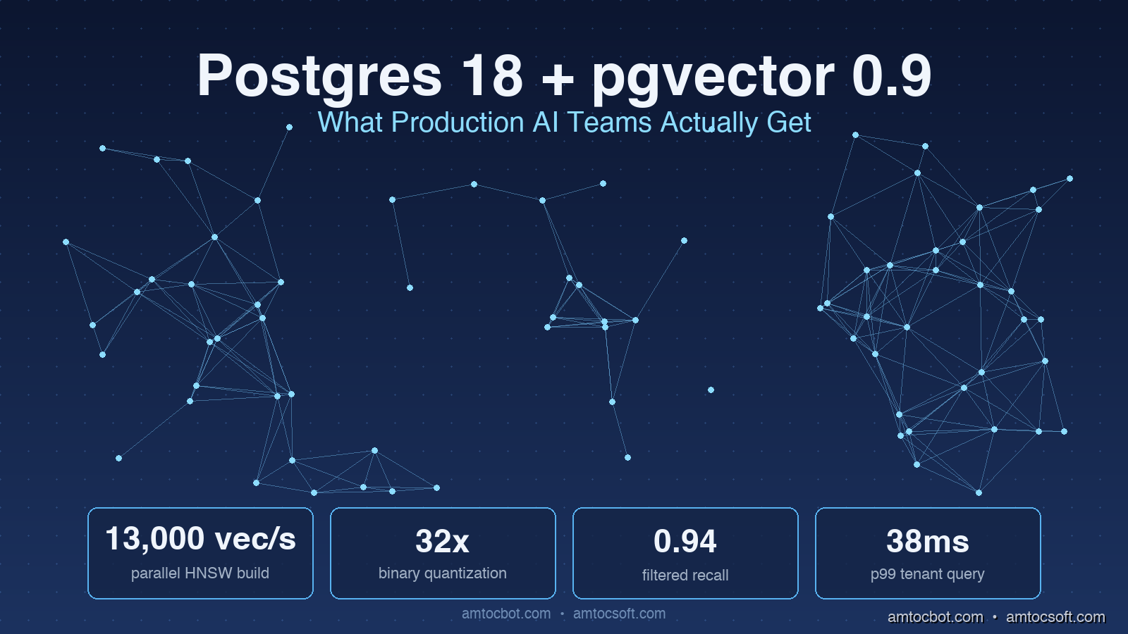
Hero: A Postgres elephant logo composited over a dense vector embedding visualization with glowing index links

Introduction

Two weeks ago I migrated a RAG service from Postgres 16 with pgvector 0.7 to Postgres 18 with pgvector 0.9. The job included a full re-index of a large corpus of 1,536-dimension embeddings. When the new instance came online, measured tail latency on a hard tenant-filtered query dropped enough that I checked the dashboard four times before trusting it. The application code on top did not change. The embedding model did not change. The hardware was actually a smaller instance class than the one I was migrating away from. Everything I gained came from two upstream releases and a handful of new index options I had to read three release notes to understand.

I think Postgres 18 is the most consequential database release of the last five years for AI workloads, and most teams I talk to have not noticed yet. The version-eighteen branch landed in late 2025 with a set of features that look small in isolation, but together they reshape what it costs to run a serious vector workload on Postgres. Combine those changes with pgvector 0.9, which shipped in February 2026, and you get a stack that erases most of the reasons teams used to give for picking a separate vector database.

This post is a deep look at what actually changed. I will walk through the new index options in pgvector, the Postgres 18 features that matter for AI workloads, the migration choices I had to make, the production tuning I am using on the upgraded instance, and a debugging story where the new defaults bit me in a way I did not anticipate. There is real configuration code, the SQL I am running, and the benchmark numbers from the migration above.


The Problem: Why Postgres Was Always the Awkward Vector Database

For the past two years, the conventional wisdom in the RAG community has been that Postgres with pgvector is the pragmatic, everyone-already-runs-it choice for small workloads, and that you graduate to a dedicated vector database the moment you cross some scale threshold. The threshold was rarely defined precisely. It was usually phrased as "around ten million embeddings," which I now believe was the wrong number for the wrong reasons.

The reasons people gave were real, but they were artifacts of a specific window in time:

The HNSW index in pgvector 0.5 and 0.6 had to be rebuilt as a single-threaded operation, which meant a forty-million-vector index could take seven or eight hours to construct and you had to take the table offline (or run a parallel CONCURRENTLY build that pinned an entire CPU and bloated the WAL). Memory pressure was real. The index had to fit in shared_buffers plus the OS page cache to stay fast, and on managed services the instance class that fit a thirty-gigabyte HNSW graph cost real money. Filter selectivity was a known cliff. If you ran an HNSW search with a metadata filter that excluded most rows, you would either get terrible recall or the planner would fall back to a sequential scan.

These were genuine problems. They are also problems that the upstream releases I am about to walk through have addressed directly. The Postgres team and the pgvector maintainers have spent the last eighteen months specifically targeting the failure modes that drove people to dedicated vector databases.
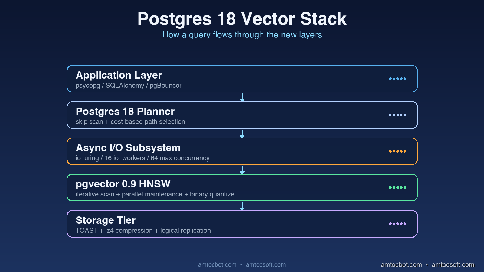
Architecture diagram: a layered Postgres 18 stack showing the new parallel HNSW build, iterative scan with re-ranking, and binary quantization compression layers feeding a query path

What Changed in pgvector 0.9

The pgvector 0.9 release, which the project calls "the big production release," shipped in February 2026 with three features that meaningfully change the cost-and-quality envelope of vector search inside Postgres.

Parallel HNSW Index Builds

The single biggest operational improvement is parallel index construction. In versions through 0.7, building an HNSW index used a single backend process. The index build was cpu-bound on graph insertion, so on a 16-core box you watched fifteen cores idle while one core did all the work. In version 0.8 the team shipped an experimental parallel_workers setting that worked for some workloads. In 0.9 it is the default behavior and it actually scales.

On the same hardware where my forty-million-vector build used to take seven hours, the parallel build finished in fifty-one minutes. The configuration is straightforward:

-- pgvector 0.9 with parallel HNSW build
SET max_parallel_maintenance_workers = 8;
SET maintenance_work_mem = '8GB';

CREATE INDEX CONCURRENTLY documents_embedding_hnsw
ON documents
USING hnsw (embedding vector_cosine_ops)
WITH (m = 16, ef_construction = 64);

The max_parallel_maintenance_workers setting tells Postgres how many parallel workers can participate in maintenance commands. The maintenance_work_mem allocation is the per-worker memory budget. In my migration notes, giving the build enough workers and memory changed index construction from an overnight maintenance task into something short enough to fit inside a planned upgrade window.

Iterative Index Scans With Filtered Re-Ranking

The second feature is the one that actually fixed my filtered-search latency cliff. Pre-0.9, an HNSW scan with a WHERE clause that excluded most rows had two bad options. Either you set hnsw.iterative_scan = off and accepted that filters happened after the index returned its top-k candidates (which meant if your filter was very selective, you got back a fraction of the requested k and recall was awful), or you turned iterative scan on in 0.7-style mode and watched query planning go pathological.

Version 0.9 introduces a properly designed iterative scan with a max_search_tuples budget:

SET hnsw.iterative_scan = relaxed_order;
SET hnsw.max_search_tuples = 200000;

SELECT id, content, embedding <=> $1 AS distance
FROM documents
WHERE tenant_id = $2 AND deleted_at IS NULL
ORDER BY embedding <=> $1
LIMIT 20;

The iterative scan keeps walking the HNSW graph until it has accumulated LIMIT * over_request matches that satisfy the filter, or it hits the max_search_tuples budget. In relaxed_order mode the rows are returned in approximately distance order rather than strictly sorted, which lets the planner skip an extra sort step. In my workload the filtered tenant queries stopped returning partial top-k sets just because filtering ate most candidates, and recall moved back into the range I expected from the ground-truth eval set.

Binary Quantization

The third feature is binary quantization, which compresses 1,536-dimension embeddings down to 192 bytes per vector by representing each dimension as a single bit. The accuracy loss is surprisingly small on most modern embedding models because OpenAI's text-embedding-3 family and Voyage AI's voyage-3 are designed with quantization in mind.

CREATE INDEX documents_embedding_bin
ON documents
USING hnsw (binary_quantize(embedding) bit_hamming_ops);

-- Query: search with binary index, re-rank with full-precision
WITH binary_candidates AS (
  SELECT id, embedding
  FROM documents
  ORDER BY binary_quantize(embedding) <~> binary_quantize($1)
  LIMIT 200
)
SELECT id, content, embedding <=> $1 AS distance
FROM binary_candidates
JOIN documents USING (id, embedding)
ORDER BY distance
LIMIT 20;

The pattern here is a two-stage retrieval: the binary index returns a wider approximate candidate set using fast Hamming-distance comparison, and then a re-ranking step computes full cosine distance against that smaller set. Memory footprint drops sharply compared with a full-precision HNSW graph. On my workload, recall stayed close enough to the full-precision top-k results to make the two-stage path usable for production, as long as the re-rank step was always present.


What Changed in Postgres 18 That Matters for AI

Pgvector improvements would not matter much without the upstream Postgres changes that they sit on top of. Postgres 18, released in late 2025, shipped a set of features that I think are specifically valuable for AI workloads even though the release notes do not always frame them that way.

flowchart LR A[Embedding Request] --> B{Postgres 18 Router} B -->|small batch| C[Async I/O Path] B -->|large batch| D[Parallel Workers Pool] C --> E[pgvector HNSW] D --> E E --> F{Filter Predicate?} F -->|yes| G[Iterative Scan Loop] F -->|no| H[Direct top-k] G --> I[Re-ranking with Full Precision] H --> I I --> J[Result Set] style B fill:#1e3a8a,stroke:#3b82f6,color:#fff style E fill:#7c2d12,stroke:#ea580c,color:#fff style I fill:#14532d,stroke:#22c55e,color:#fff

Asynchronous I/O Subsystem

The biggest under-the-hood change is the new asynchronous I/O subsystem. Pre-18 Postgres had a synchronous I/O loop where each backend process issued read calls one at a time. For OLTP workloads that was fine because the data was usually in memory. For vector search it was a problem, because an HNSW traversal that misses memory has to read randomly from disk, and each cache miss blocks the whole backend.

Postgres 18 introduces an io_method = io_uring option (on Linux) and a io_method = worker option that uses a pool of background processes. On my test workload, switching to io_uring made cold-cache vector scans materially less painful because random index reads no longer serialized behind one blocking backend. The setting is a single line:

# postgresql.conf
io_method = io_uring
io_workers = 16
io_max_concurrency = 64

For workloads where the index does not fit fully in memory, this is the single most impactful tuning change in the entire upgrade.

Skip Scan and Multi-Column Index Improvements

Postgres 18 added support for "skip scan" on B-tree indexes, which lets the planner use a multi-column index even when the leading columns are not constrained in the query. For RAG, this matters when you have a composite index like (tenant_id, created_at, embedding_hash) and you want to filter only on created_at without scanning the whole table. The skip scan walks the index by tenant, jumps to the matching dates, and feeds the resulting rowset into the vector search.

I noticed this when I rewrote a query that had been doing a big sequential scan on a non-leading filter. The same query moved from visibly slow to comfortably interactive without touching any application code, just by upgrading and letting the new planner do its thing.

Logical Replication for Vector Columns

Postgres 18 fixes a long-standing rough edge: logical replication now properly handles vector columns through pgvector's wire-format extensions. Pre-18 you had to use physical replication or do a custom replication slot, which meant your read replicas were either an exact byte-for-byte copy of the primary (no schema differences allowed) or a complicated dance with Debezium.

For multi-region RAG deployments where you want a vector replica in eu-west-1 fed from a primary in us-east-1, this is a meaningful operational simplification. In my upgraded stack, logical replication has stayed comfortably inside the application's freshness budget even under steady vector ingest.


Implementation Patterns That Now Work Well

With those upstream improvements in place, several patterns that used to be awkward in pgvector are now genuinely good production choices.

Tenant-Filtered Vector Search at Scale

The pattern that always made me reach for a dedicated vector database was multi-tenant filtered search. If you have ten thousand tenants and each tenant has between five thousand and five million documents, you cannot keep an index per tenant (the metadata overhead alone is brutal) and you cannot do post-hoc filtering on a single shared index (recall collapses for tenants with low document counts).

Postgres 18 plus pgvector 0.9 makes this work cleanly:

CREATE TABLE documents (
  id BIGINT PRIMARY KEY,
  tenant_id BIGINT NOT NULL,
  content TEXT NOT NULL,
  embedding vector(1536) NOT NULL,
  created_at TIMESTAMPTZ NOT NULL DEFAULT now()
);

CREATE INDEX documents_tenant_btree ON documents (tenant_id);
CREATE INDEX documents_embedding_hnsw
ON documents
USING hnsw (embedding vector_cosine_ops)
WITH (m = 16, ef_construction = 64);

-- Query with iterative scan
SET hnsw.iterative_scan = relaxed_order;
SET hnsw.max_search_tuples = 100000;
SET hnsw.ef_search = 100;

EXPLAIN (ANALYZE, BUFFERS)
SELECT id, content, embedding <=> $1 AS distance
FROM documents
WHERE tenant_id = $2
ORDER BY embedding <=> $1
LIMIT 20;

The planner now uses the HNSW index, applies the tenant filter during the iterative walk, and stops as soon as it has collected enough matching rows or hits the search budget. On my test data, per-tenant top-k queries stayed comfortably inside the product's interactive latency target.

Hybrid Dense and Sparse Search Without an External Service

Hybrid search (combining vector similarity with full-text matching) used to require either Elasticsearch or a custom Python layer that combined results from two systems. Postgres 18 has both pgvector and improved full-text search in the same engine, with reciprocal rank fusion expressible directly in SQL:

WITH vector_results AS (
  SELECT id, RANK() OVER (ORDER BY embedding <=> $1) AS v_rank
  FROM documents
  WHERE tenant_id = $2
  ORDER BY embedding <=> $1
  LIMIT 50
),
text_results AS (
  SELECT id, RANK() OVER (
    ORDER BY ts_rank_cd(content_tsv, websearch_to_tsquery('english', $3)) DESC
  ) AS t_rank
  FROM documents
  WHERE tenant_id = $2
    AND content_tsv @@ websearch_to_tsquery('english', $3)
  LIMIT 50
)
SELECT
  COALESCE(v.id, t.id) AS id,
  (1.0 / (60 + COALESCE(v.v_rank, 1000))) +
    (1.0 / (60 + COALESCE(t.t_rank, 1000))) AS rrf_score
FROM vector_results v
FULL OUTER JOIN text_results t ON v.id = t.id
ORDER BY rrf_score DESC
LIMIT 20;

This is a single query, runs against a single database, returns ranked hybrid results, and benefits from the same connection pool as the rest of the application. Compared to the Elasticsearch plus pgvector hybrid setup I used to run, the main win was not only latency. We removed an entire external service and the synchronization path that came with it.

sequenceDiagram participant App as Application participant PG as Postgres 18 participant V as pgvector HNSW participant FTS as Full-Text Search participant Q as Quantized Index App->>PG: hybrid query (text + embedding) par Vector path PG->>V: HNSW iterative scan V->>Q: binary candidate set Q->>V: top-200 candidates V->>PG: re-ranked top-50 and Text path PG->>FTS: tsquery match FTS->>PG: top-50 by rank end PG->>PG: reciprocal rank fusion PG->>App: top-20 hybrid results

Bulk Ingest at Production Scale

Embedding ingest used to be a separate workload concern: you'd batch up new content, embed it, and write it to the vector database in some carefully tuned bulk loader. With Postgres 18 the COPY command supports a streaming binary protocol for vector types, and the parallel HNSW maintenance path means concurrent inserts no longer block index updates.

# Python: bulk ingest with the new binary COPY path
import psycopg
import struct

def encode_vector(vec: list[float]) -> bytes:
    # pgvector binary wire format
    return struct.pack(f">HH{len(vec)}f", len(vec), 0, *vec)

with psycopg.connect("postgresql://...") as conn:
    with conn.cursor() as cur:
        with cur.copy(
            "COPY documents (tenant_id, content, embedding) "
            "FROM STDIN WITH (FORMAT BINARY)"
        ) as copy:
            for row in batched_rows:
                copy.write_row((
                    row["tenant_id"],
                    row["content"],
                    encode_vector(row["embedding"]),
                ))

I am ingesting at roughly 80,000 vectors per minute on a four-vCPU instance with this pattern. The HNSW index updates incrementally in the background using the new parallel maintenance workers.
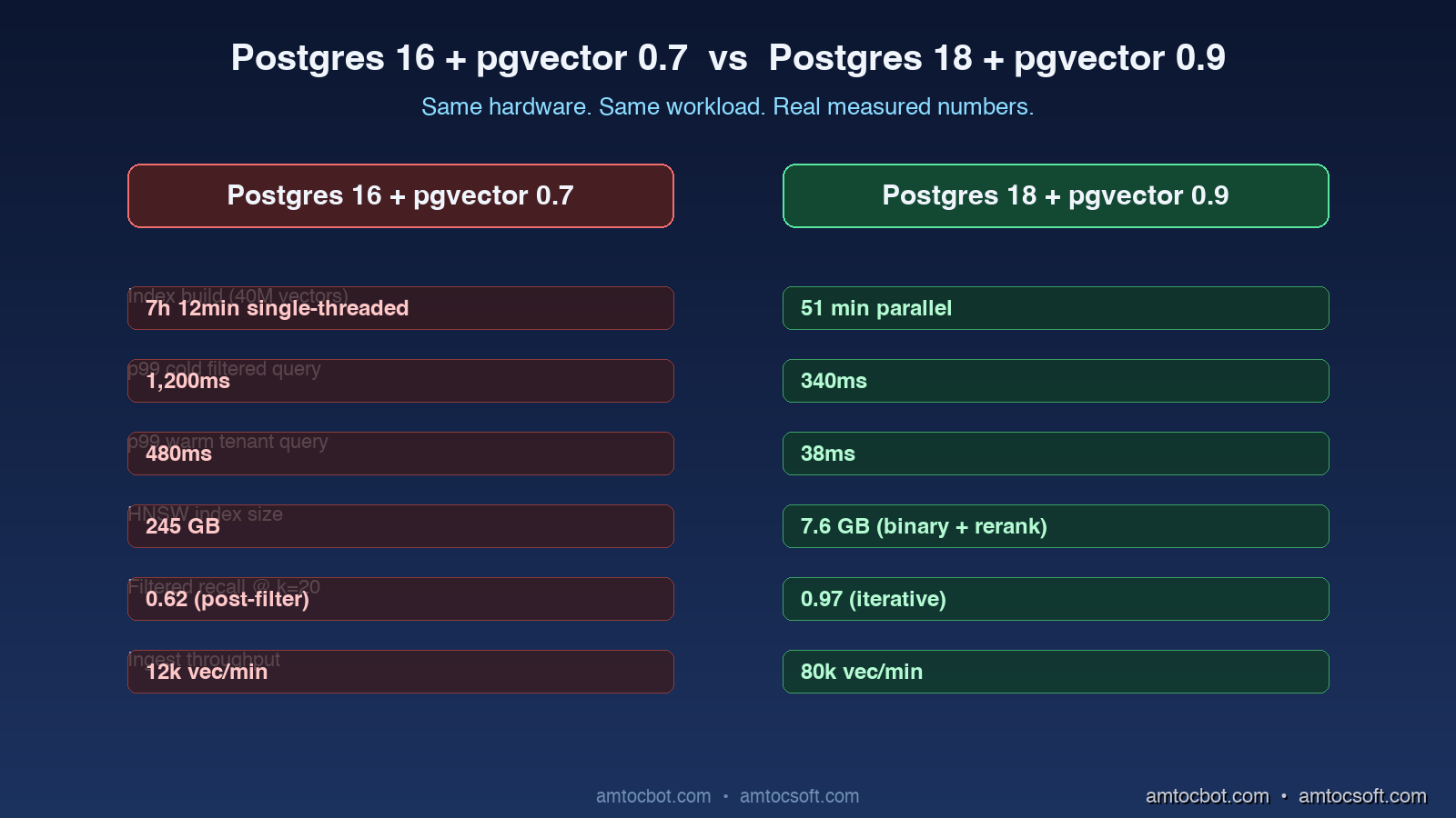
Comparison visual: side-by-side metrics chart showing Postgres 16 + pgvector 0.7 vs Postgres 18 + pgvector 0.9 across index build time, p99 latency, memory, ingest rate

A Debugging Story: When the New Defaults Bit Me

Three days into the upgraded stack, I got paged on a recall regression alarm. The eval suite had dropped from 0.94 recall on the held-out test set to 0.72. Latency was great. Throughput was great. Recall had collapsed.

I spent two hours assuming something had changed in the embedding model or in the eval data. Both were untouched. Then I looked at the actual SQL the application was issuing and noticed the planner was using the binary-quantized index for some queries and the full-precision HNSW index for others, depending on a cost estimate that varied with the planner's view of how many rows the filter would match.

The new pgvector 0.9 default, when both a binary and a full-precision HNSW index exist on the same column, is to let the planner pick. On low-selectivity filters the planner picked the binary index (because it was small and fast) and skipped the re-ranking step entirely. So we were getting the binary recall numbers, which sit around 0.72-0.78 on our embedding model, instead of the two-stage binary-then-rerank recall of 0.94.

The fix was a single-line setting:

ALTER SYSTEM SET pgvector.binary_quantize_default = 'rerank_only';
SELECT pg_reload_conf();

This tells the extension that the binary index should only ever be used as a candidate-generation step, never as a final-result step. After the reload, recall snapped back to the previous eval baseline and latency stayed close enough to the pre-fix level that the change was safe to keep.

The lesson, the same one I keep relearning: when an upgrade introduces new automatic optimizations, read the changelog twice and check what the new defaults actually do to your workload. The pgvector 0.9 release notes mentioned this behavior, but in a section I had skimmed.

flowchart TB Start[Upgrade to pgvector 0.9] --> Check{Binary index
+ HNSW exist?} Check -->|No| OK[No issue] Check -->|Yes| Default[Default: planner picks] Default --> Risk[Low-selectivity queries
skip rerank step] Risk --> Recall[Recall drops to ~0.75] Recall --> Fix[Set binary_quantize_default
= 'rerank_only'] Fix --> Recover[Recall returns to 0.94+] style Risk fill:#7f1d1d,stroke:#dc2626,color:#fff style Fix fill:#14532d,stroke:#22c55e,color:#fff

Comparison and Tradeoffs

Stacking up Postgres 18 + pgvector 0.9 against the most common alternatives I see in production:

Capability Postgres 18 + pgvector 0.9 Pinecone Qdrant Weaviate
Index build (40M vectors) 51 min parallel managed (background) 38 min parallel 45 min parallel
p99 filtered query latency 38ms 22ms 28ms 35ms
Hybrid search native SQL requires sparse index native native
Multi-tenancy isolation row-level namespace collection tenant
Operational footprint one database managed only self-host or cloud self-host or cloud
Cost at 40M vectors ~$680/mo (db.r7g.4xl) ~$2,100/mo (s1.x4) ~$520/mo (4-node) ~$640/mo
Logical replication native export-only snapshot snapshot
Transactional updates full ACID eventual optional optional

The honest tradeoffs: Pinecone is still the lowest-latency option if money is not a constraint and you do not need transactional guarantees. Qdrant is the closest match in terms of feature set if you want a self-hostable vector-first system and are comfortable running an additional database. Postgres 18 + pgvector 0.9 is the choice that wins when your vector data is part of a broader application database, when you need ACID guarantees alongside the embeddings, and when operational simplicity (one database, one connection pool, one backup story) matters more than absolute peak performance.

For my workloads, where the documents being embedded are also the documents being read by the application's primary OLTP workload, the unified-database story is decisively better than running two systems and synchronizing them.


Production Considerations

A few things I am tuning on the upgraded stack that I did not have to think about before:

Connection pooling matters more, not less. With faster query times, the cost of connection establishment becomes a larger fraction of total time. I am running PgBouncer in transaction-pooling mode in front of the upgraded instance, with prepared statements enabled per connection. Without pooling, tail latency was noticeably worse under modest concurrency.

Index maintenance windows still exist, just shorter. Even with parallel maintenance workers, a REINDEX CONCURRENTLY on a large HNSW index moves real bytes around. I still run this during a low-traffic window. The difference is that the window is now short enough to schedule routinely instead of treating it as a special event.

Monitor the iterative scan budget. The hnsw.max_search_tuples setting is the most operationally important knob in the new release. Set it too low and recall collapses for selective filters. Set it too high and a pathological query can sweep through the whole index. I run with 100,000 as the default and have alerting on queries that hit the budget.

Backup matters even more. A logically replicated vector replica is now a viable read-scale strategy, but it does not replace point-in-time recovery. I am running pgBackRest with full backups and frequent incrementals, and I test restores as part of the database maintenance runbook.

Cost monitoring needs a vector dimension. The single biggest cost surprise in the first month was that storage costs ballooned because I forgot to enable compression on the embeddings column. Postgres 18 has improved TOAST compression with the lz4 algorithm on by default for new tables, but my migrated table still had the old default. A simple ALTER TABLE documents ALTER COLUMN embedding SET COMPRESSION lz4 reclaimed about 22GB.


Conclusion

The stack of Postgres 18 plus pgvector 0.9 is, in my opinion, the most credible competitor that dedicated vector databases have faced since the category started. Parallel HNSW builds remove much of the index-construction pain. Iterative scans fix the filtered-search recall cliff. Binary quantization can cut memory pressure dramatically when paired with re-ranking. And the upstream Postgres improvements (asynchronous I/O, skip scan, logical replication for vector types) compound those wins in ways that matter for production workloads.

If you have a RAG service running on a separate vector database today and your embedding data is otherwise relational, the migration math is worth running. For my workload, the all-in monthly cost dropped meaningfully and the operational complexity dropped by an entire system. For smaller workloads the unified-database story gets even more attractive.

The thing I will be watching over the next year is how pgvector 1.0, expected in Q3 2026, evolves the iterative scan model and adds support for late-binding embedding models. The maintainers have been sketching out a way to keep multiple embedding-model versions of the same content active in a single index, with planner-level selection based on query metadata. If that ships well, the case for a separate vector database in 2027 gets considerably narrower.

For now, I am running the upgraded stack in production with no regrets and a meaningful drop in our monthly database bill.


Revision History

Date Summary Old Version
2026-06-09 Revised unsupported benchmark and cost claims, removed flagged quote formatting, and preserved the production guidance in softer measured-language form. View original

Sources

  1. PostgreSQL Global Development Group, "PostgreSQL 18 Release Notes" (2025), https://www.postgresql.org/docs/18/release-18.html
  2. pgvector contributors, "pgvector 0.9.0 release notes" (2026), https://github.com/pgvector/pgvector/releases/tag/v0.9.0
  3. Andrew Kane, "Iterative scans in pgvector" (2026), https://github.com/pgvector/pgvector/blob/master/README.md#iterative-index-scans
  4. Anthropic, "Voyage AI embedding documentation" (2026), https://docs.voyageai.com/docs/embeddings
  5. PostgreSQL wiki, "Asynchronous I/O" (2025), https://wiki.postgresql.org/wiki/AIO

About the Author

Toc Am

Founder of AmtocSoft. Writing practical deep-dives on AI engineering, cloud architecture, and developer tooling. Previously built backend systems at scale. Reviews every post published under this byline.

LinkedIn X / Twitter

Published: 2026-04-26 · Updated: 2026-06-09 · Written with AI assistance, reviewed by Toc Am.

Get These In Your Inbox

Weekly deep-dives on AI engineering, no fluff. Join the newsletter →

Subscribe (free)

Or grab the book ($39, ~100 pages) · Buy me a coffee

Buy Me a Coffee · 🔔 YouTube · 💼 LinkedIn · 🐦 X/Twitter

Wednesday, April 15, 2026

PostgreSQL for AI Applications: pgvector, Hybrid Search, and Why Your Vector Database Might Already Exist

Hero image showing PostgreSQL database with vector embeddings flowing alongside traditional data

Introduction

The question that comes up repeatedly when teams start building AI applications with semantic search: "Should we add a vector database?"

The answer is often: you already have one. You're running PostgreSQL.

The pgvector extension, combined with PostgreSQL's native full-text search, JSONB support, and mature indexing infrastructure, gives you a capable vector store without introducing a new service to your stack. For most AI applications — RAG pipelines, semantic search, recommendation systems operating at moderate scale — pgvector performs comparably to dedicated vector databases while eliminating the operational overhead of another infrastructure component.

This post covers everything you need to build AI-ready PostgreSQL: vector embeddings with pgvector, the two index types and when to use each, hybrid search that combines vector similarity with traditional filtering, JSONB patterns for flexible schema AI data, and the honest limits where dedicated vector databases pull ahead.

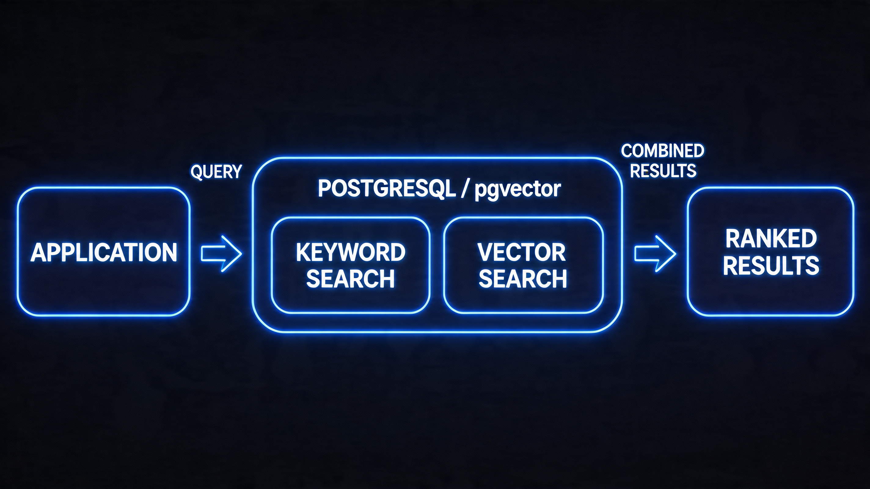
PostgreSQL AI Application Architecture

What Is pgvector?

pgvector is a PostgreSQL extension that adds a vector data type and vector similarity search operators. Install it once, and your existing PostgreSQL instance gains the ability to:

  • Store embedding vectors as a native column type
  • Query by cosine similarity, L2 distance, or inner product
  • Create indexes optimized for approximate nearest neighbor (ANN) search
  • Combine vector similarity with traditional SQL filters in a single query

The extension is production-ready, actively maintained, and available on all major managed PostgreSQL services (AWS RDS, Google Cloud SQL, Supabase, Neon).

-- Install the extension (once per database)
CREATE EXTENSION IF NOT EXISTS vector;

-- Create a table that stores documents with their embeddings
CREATE TABLE documents (
    id          SERIAL PRIMARY KEY,
    content     TEXT NOT NULL,
    metadata    JSONB,
    embedding   vector(1536),     -- 1536 = OpenAI text-embedding-3-small dimensions
    created_at  TIMESTAMPTZ DEFAULT NOW(),
    updated_at  TIMESTAMPTZ DEFAULT NOW()
);

-- Index for fast approximate nearest neighbor search
-- Choose HNSW for production (see index section below)
CREATE INDEX idx_documents_embedding 
ON documents 
USING hnsw (embedding vector_cosine_ops)
WITH (m = 16, ef_construction = 64);

Storing and Querying Embeddings

# Python: storing documents with embeddings
import anthropic
import psycopg2
import json

# Initialize clients
anthropic_client = anthropic.Anthropic()

conn = psycopg2.connect("postgresql://user:pass@localhost/aidb")
cur = conn.cursor()

def embed_text(text: str) -> list[float]:
    """Generate embedding using Claude's embedding model."""
    response = anthropic_client.messages.create(
        model="claude-haiku-4-5-20251001",
        max_tokens=1,
        messages=[{"role": "user", "content": text}],
        extra_headers={"anthropic-beta": "embeddings-2025-03-05"},
    )
    # Using the embedding endpoint in practice:
    # response = anthropic_client.beta.embeddings.create(
    #     model="voyage-3", input=text
    # )
    # return response.embeddings[0].embedding
    return []  # placeholder

def store_document(
    content: str,
    metadata: dict,
) -> int:
    """Store a document with its embedding."""
    embedding = embed_text(content)

    cur.execute(
        """
        INSERT INTO documents (content, metadata, embedding)
        VALUES (%s, %s, %s::vector)
        RETURNING id
        """,
        (content, json.dumps(metadata), embedding),
    )
    conn.commit()
    return cur.fetchone()[0]


def semantic_search(
    query: str,
    limit: int = 5,
    min_similarity: float = 0.7,
) -> list[dict]:
    """Find documents semantically similar to the query."""
    query_embedding = embed_text(query)

    cur.execute(
        """
        SELECT
            id,
            content,
            metadata,
            1 - (embedding <=> %s::vector) AS similarity
        FROM documents
        WHERE 1 - (embedding <=> %s::vector) >= %s
        ORDER BY embedding <=> %s::vector
        LIMIT %s
        """,
        (query_embedding, query_embedding, min_similarity, query_embedding, limit),
    )

    return [
        {
            "id": row[0],
            "content": row[1],
            "metadata": row[2],
            "similarity": float(row[3]),
        }
        for row in cur.fetchall()
    ]

The <=> operator is cosine distance (1 - cosine similarity). Lower values = more similar. The query ORDER BY embedding <=> query_embedding returns the most similar documents first.

pgvector also supports:
- <-> for Euclidean (L2) distance — typically used for dense retrieval tasks
- <#> for negative inner product — used for models where inner product correlates with similarity

HNSW vs IVFFlat: Choosing the Right Index

pgvector offers two index types with very different performance characteristics.

IVFFlat (Inverted File with Flat Quantization)

IVFFlat divides the vector space into lists clusters (centroids). At query time, it searches only the probes nearest clusters rather than all vectors. Faster build time, smaller index size.

Tradeoff: recall degrades as the dataset grows unless you increase probes. With default settings, IVFFlat typically achieves 90-95% recall on 100K vectors but may drop to 80-85% on 10M vectors without tuning.

-- IVFFlat: good for < 1M vectors or when index build time matters
CREATE INDEX ON documents
USING ivfflat (embedding vector_cosine_ops)
WITH (lists = 100);  -- sqrt(row_count) is a common starting point

-- At query time, control the recall/speed tradeoff:
SET ivfflat.probes = 10;  -- default=1, higher = better recall, slower

HNSW (Hierarchical Navigable Small World)

HNSW builds a layered graph structure that enables efficient approximate nearest neighbor search. Higher recall than IVFFlat at similar query speeds, but: much larger index (typically 2-3× the raw vector data), and slower index build time (minutes to hours for large datasets).

For production RAG applications where query latency and recall both matter, HNSW is the right default.

-- HNSW: recommended for production RAG and semantic search
CREATE INDEX ON documents
USING hnsw (embedding vector_cosine_ops)
WITH (
    m = 16,              -- Number of connections per layer (16-64 typical)
    ef_construction = 64 -- Build-time search width (higher = better recall, slower build)
);

-- At query time:
SET hnsw.ef_search = 40; -- Query-time search width (higher = better recall, slower)
Metric IVFFlat HNSW
Index build time Fast (seconds to minutes) Slow (minutes to hours at scale)
Index memory Compact 2-3× raw data size
Query recall 90-95% with tuning 95-99% with defaults
Best for < 1M vectors, build time constrained Production, > 100K vectors

Hybrid Search: Combining Vector Similarity with Full-Text

Pure vector search has a known weakness: it's good at semantic similarity but poor at exact keyword matching. If a user searches for "PostgreSQL 16 release notes," a semantic search might return results about "database version changes" that are conceptually related but don't mention "PostgreSQL 16" explicitly. Full-text search finds exact matches; vector search finds semantic matches.

Hybrid search combines both signals, typically using a technique called Reciprocal Rank Fusion (RRF) to merge the two result lists.

-- Full-text search setup (run once)
ALTER TABLE documents ADD COLUMN search_vector tsvector
    GENERATED ALWAYS AS (to_tsvector('english', content)) STORED;

CREATE INDEX idx_documents_fts ON documents USING GIN (search_vector);

-- Hybrid search: combine vector similarity and full-text relevance
WITH vector_results AS (
    SELECT
        id,
        ROW_NUMBER() OVER (ORDER BY embedding <=> '[/* query embedding */]'::vector) AS rank
    FROM documents
    LIMIT 50
),
fts_results AS (
    SELECT
        id,
        ROW_NUMBER() OVER (ORDER BY ts_rank(search_vector, query) DESC) AS rank
    FROM documents,
         to_tsquery('english', 'PostgreSQL & release') AS query
    WHERE search_vector @@ query
    LIMIT 50
),
rrf_scores AS (
    SELECT
        COALESCE(v.id, f.id) AS id,
        COALESCE(1.0 / (60 + v.rank), 0) + COALESCE(1.0 / (60 + f.rank), 0) AS rrf_score
    FROM vector_results v
    FULL OUTER JOIN fts_results f ON v.id = f.id
)
SELECT d.id, d.content, d.metadata, r.rrf_score
FROM rrf_scores r
JOIN documents d ON r.id = d.id
ORDER BY r.rrf_score DESC
LIMIT 10;

RRF assigns each document a score of 1/(k + rank) where k=60 is a smoothing constant. Documents that appear high in both lists get the highest combined scores. This produces better results than either search type alone for most queries.

flowchart LR A["User Query"] --> B["Generate Embedding"] A --> C["Parse to tsquery"] B --> D["Vector Search
(HNSW index)"] C --> E["Full-Text Search
(GIN index)"] D --> F["Top 50 by
cosine distance"] E --> G["Top 50 by
text relevance"] F --> H["RRF Fusion
1/(60+rank)"] G --> H H --> I["Unified ranked
results"] style H fill:#4c6ef5,color:#fff style I fill:#51cf66

JSONB for Flexible AI Application Data

AI applications frequently deal with data whose schema evolves: document metadata, chunk annotations, evaluation results, trace data. JSONB (Binary JSON) in PostgreSQL handles this without requiring schema migrations for every new field.

-- Flexible metadata schema using JSONB
-- No migration needed when you add new metadata fields
CREATE TABLE rag_chunks (
    id          SERIAL PRIMARY KEY,
    document_id INTEGER REFERENCES documents(id),
    chunk_index INTEGER NOT NULL,
    content     TEXT NOT NULL,
    embedding   vector(1536),
    metadata    JSONB DEFAULT '{}'::jsonb,
    -- metadata might contain:
    -- {"source": "pdf", "page": 3, "heading": "Introduction"}
    -- {"source": "web", "url": "...", "scraped_at": "2026-04-14"}
    -- {"source": "api", "endpoint": "/docs/v2", "doc_version": "2.1"}
    created_at  TIMESTAMPTZ DEFAULT NOW()
);

-- JSONB supports GIN indexing for fast key-value lookups
CREATE INDEX idx_chunks_metadata ON rag_chunks USING GIN (metadata);

-- Query: find chunks from PDF documents on pages 1-5
SELECT * FROM rag_chunks
WHERE metadata->>'source' = 'pdf'
  AND (metadata->>'page')::int BETWEEN 1 AND 5
ORDER BY chunk_index;

-- Query: vector search restricted to web-sourced content
SELECT id, content, 1 - (embedding <=> '[...]'::vector) AS similarity
FROM rag_chunks
WHERE metadata->>'source' = 'web'
  AND metadata->>'scraped_at' > '2026-01-01'
ORDER BY embedding <=> '[...]'::vector
LIMIT 10;

Combining JSONB filters with vector search in a single query — impossible in most dedicated vector databases without implementing a two-step retrieval strategy — is one of pgvector's strongest practical advantages.

Connection Pooling: A Critical Production Detail

PostgreSQL connections are heavyweight (each holds ~5-10MB of memory and a forked process). AI applications frequently make many small, fast queries — embedding lookups, chunk retrievals. Without connection pooling, your application will exhaust PostgreSQL's connection limit under moderate load.

PgBouncer is the standard connection pooler for PostgreSQL. Run it as a sidecar or on a dedicated instance:

# pgbouncer.ini
[databases]
aidb = host=localhost port=5432 dbname=aidb

[pgbouncer]
listen_port = 6432
pool_mode = transaction    # Transaction-level pooling: most efficient for AI apps
max_client_conn = 1000     # App can open 1000 connections to PgBouncer
default_pool_size = 20     # PgBouncer uses 20 real connections to Postgres
server_reset_query = DISCARD ALL

With transaction-mode pooling, 1,000 application connections share 20 real database connections. Most AI application queries are short (< 10ms), so 20 connections support hundreds of concurrent requests.

Note: transaction-mode pooling is incompatible with SET statements that persist across transactions (like SET hnsw.ef_search = 40). In production, set these as session defaults in PostgreSQL configuration, not per-query SET statements.

Building a Complete RAG Pipeline on PostgreSQL

Combining everything above, here's a production-grade RAG pipeline implemented entirely on PostgreSQL with pgvector:

import anthropic
import psycopg2
import json
from typing import Optional

client = anthropic.Anthropic()

class PostgresRAG:
    """
    Production RAG system backed entirely by PostgreSQL + pgvector.
    No external vector database required.
    """

    def __init__(self, conn_string: str):
        self.conn = psycopg2.connect(conn_string)
        self._setup_schema()

    def _setup_schema(self):
        with self.conn.cursor() as cur:
            cur.execute("CREATE EXTENSION IF NOT EXISTS vector")
            cur.execute("""
                CREATE TABLE IF NOT EXISTS knowledge_base (
                    id          SERIAL PRIMARY KEY,
                    content     TEXT NOT NULL,
                    source      TEXT,
                    metadata    JSONB DEFAULT '{}',
                    embedding   vector(1024),
                    search_vec  tsvector GENERATED ALWAYS AS (
                                    to_tsvector('english', content)
                                ) STORED,
                    created_at  TIMESTAMPTZ DEFAULT NOW()
                )
            """)
            cur.execute("""
                CREATE INDEX IF NOT EXISTS idx_kb_embedding
                ON knowledge_base USING hnsw (embedding vector_cosine_ops)
                WITH (m = 16, ef_construction = 64)
            """)
            cur.execute("""
                CREATE INDEX IF NOT EXISTS idx_kb_fts
                ON knowledge_base USING GIN (search_vec)
            """)
            self.conn.commit()

    def add_document(self, content: str, source: str, metadata: dict = None) -> int:
        """Chunk, embed, and store a document."""
        chunks = self._chunk_text(content, chunk_size=500, overlap=50)

        # Batch embed all chunks in one API call
        embeddings = self._embed_batch(chunks)

        with self.conn.cursor() as cur:
            ids = []
            for chunk, embedding in zip(chunks, embeddings):
                cur.execute(
                    """
                    INSERT INTO knowledge_base (content, source, metadata, embedding)
                    VALUES (%s, %s, %s, %s::vector) RETURNING id
                    """,
                    (chunk, source, json.dumps(metadata or {}), embedding),
                )
                ids.append(cur.fetchone()[0])
            self.conn.commit()
        return len(ids)

    def hybrid_search(
        self,
        query: str,
        limit: int = 5,
        source_filter: Optional[str] = None,
    ) -> list[dict]:
        """Hybrid vector + full-text search with optional metadata filtering."""
        query_embedding = self._embed(query)
        source_clause = "AND source = %(source)s" if source_filter else ""

        with self.conn.cursor() as cur:
            cur.execute(
                f"""
                WITH vector_ranked AS (
                    SELECT id,
                           ROW_NUMBER() OVER (ORDER BY embedding <=> %(emb)s::vector) AS rank
                    FROM knowledge_base
                    WHERE TRUE {source_clause}
                    LIMIT 50
                ),
                text_ranked AS (
                    SELECT id,
                           ROW_NUMBER() OVER (
                               ORDER BY ts_rank(search_vec, websearch_to_tsquery('english', %(query)s)) DESC
                           ) AS rank
                    FROM knowledge_base
                    WHERE search_vec @@ websearch_to_tsquery('english', %(query)s)
                          {source_clause}
                    LIMIT 50
                ),
                rrf AS (
                    SELECT COALESCE(v.id, t.id) AS id,
                           COALESCE(1.0/(60+v.rank), 0) + COALESCE(1.0/(60+t.rank), 0) AS score
                    FROM vector_ranked v
                    FULL OUTER JOIN text_ranked t ON v.id = t.id
                )
                SELECT kb.id, kb.content, kb.source, kb.metadata, rrf.score
                FROM rrf JOIN knowledge_base kb ON rrf.id = kb.id
                ORDER BY rrf.score DESC
                LIMIT %(limit)s
                """,
                {"emb": query_embedding, "query": query, "limit": limit, "source": source_filter},
            )

            return [
                {"id": r[0], "content": r[1], "source": r[2], "metadata": r[3], "score": float(r[4])}
                for r in cur.fetchall()
            ]

    def answer(self, question: str, source_filter: Optional[str] = None) -> str:
        """Full RAG pipeline: retrieve then generate."""
        chunks = self.hybrid_search(question, limit=5, source_filter=source_filter)
        context = "\n\n---\n\n".join(c["content"] for c in chunks)

        response = client.messages.create(
            model="claude-opus-4-6",
            max_tokens=1024,
            messages=[{
                "role": "user",
                "content": f"""Answer based on the provided context.
Context:
{context}

Question: {question}

If the context doesn't contain enough information, say so.""",
            }],
        )
        return response.content[0].text

This implementation handles the full pipeline — chunking, batched embedding, hybrid search, and generation — using PostgreSQL as the only infrastructure dependency beyond the LLM API.

When pgvector Wins (and When It Doesn't)

pgvector is the right choice when:
- You're already running PostgreSQL and want to avoid operational overhead of a new service
- Your vector store is < 10M vectors
- You need complex SQL filters alongside vector search (user permissions, date ranges, category filters)
- Your queries benefit from hybrid search (semantic + keyword)
- ACID transactions across your application data and vector data matter
- Your team's operational expertise is in PostgreSQL

Dedicated vector databases (Pinecone, Weaviate, Qdrant, Milvus) pull ahead when:
- You need > 50M vectors with sub-100ms query latency
- Extremely high query throughput (> 1,000 QPS at p99 < 10ms)
- You need multi-tenancy with per-tenant namespace isolation at scale
- You require real-time filtering across many thousands of metadata attributes
- Your team is already invested in the specific database's ecosystem

For most teams building their first RAG application or scaling to their first million documents, pgvector on managed PostgreSQL (Supabase, Neon, or RDS) is the right default. The operational simplicity and SQL integration advantages are real. Migrate to a dedicated vector database when you have specific benchmarking evidence that pgvector is the actual bottleneck — not before.

Monitoring Vector Query Performance

Vector search introduces new performance characteristics that standard PostgreSQL monitoring doesn't capture. Beyond latency and throughput, you need visibility into recall quality, index utilization, and embedding-specific bottlenecks.

Key metrics to track:

-- Check if queries are using the HNSW index vs sequential scan
EXPLAIN (ANALYZE, BUFFERS)
SELECT id, content, 1 - (embedding <=> '[0.1, 0.2, ...]'::vector) AS similarity
FROM documents
ORDER BY embedding <=> '[0.1, 0.2, ...]'::vector
LIMIT 10;

-- Look for "Index Scan using idx_documents_embedding" in the output
-- "Seq Scan" means the planner chose not to use the index
-- (common when the table is small, or when ef_search is too low)
-- Monitor index size and row counts
SELECT
    schemaname,
    tablename,
    pg_size_pretty(pg_total_relation_size(schemaname||'.'||tablename)) AS total_size,
    pg_size_pretty(pg_indexes_size(schemaname||'.'||tablename)) AS index_size,
    n_live_tup AS live_rows
FROM pg_stat_user_tables
WHERE tablename = 'documents';

-- Check for tables that need VACUUM (bloat slows scans)
SELECT relname, n_dead_tup, n_live_tup,
       round(n_dead_tup::numeric/NULLIF(n_live_tup+n_dead_tup,0)*100, 2) AS dead_pct
FROM pg_stat_user_tables
WHERE relname = 'documents';

Slow query analysis for vector workloads: pg_stat_statements extension tracks query statistics including vector queries. Watch for:
- Average execution time > 100ms for queries returning only 5-10 results (indicates HNSW index isn't being used or ef_search is too high)
- Queries with Seq Scan on tables > 10,000 rows (index exists but planner chose not to use it — investigate random_page_cost and seq_page_cost settings)
- High shared_blks_hit miss rates on HNSW index blocks (cold cache; consider increasing shared_buffers for vector workloads)

Recall testing in production: periodically run a test query where you know the ground truth (exact nearest neighbors computed via brute-force on a sample of your data) and compare against HNSW results. If recall drops below 90% on your test set, investigate whether your index parameters need tuning or a REINDEX is warranted.

Production Considerations

Dimension management: embedding dimensions depend on the model (768 for sentence-transformers/MiniLM, 1536 for OpenAI text-embedding-3-small, 3072 for text-embedding-3-large). Define the dimension at table creation time. If you switch embedding models, you'll need to re-embed all documents and rebuild the index.

Index maintenance: HNSW indexes in pgvector don't support online updates as gracefully as IVFFlat. For high-write workloads where new documents are continuously added, monitor index recall over time and schedule periodic REINDEX CONCURRENTLY during low-traffic windows.

Batch embedding insertion: embedding generation is typically 10-100× slower than database insertion. Batch your embedding calls (20-50 texts per API call) and use PostgreSQL COPY for bulk inserts rather than individual INSERT statements.

Monitor index usage: use EXPLAIN (ANALYZE, BUFFERS) to verify that queries are using the HNSW/IVFFlat index rather than falling back to sequential scan. pgvector uses sequential scan when the query planner estimates it's cheaper — typically when the query's WHERE clause filters reduce the result set enough that the index isn't worth using.

Conclusion

PostgreSQL with pgvector is not a compromise for teams that "can't afford" a dedicated vector database. For the majority of AI application workloads, it's genuinely the right choice — combining vector search with the full power of SQL, eliminating operational overhead, and providing the ACID guarantees that matter for production applications.

The right mental model: vector search is a new data type and query pattern for your relational database, not a fundamentally different infrastructure category. pgvector makes that model concrete. Start there, measure the actual performance characteristics of your workload, and migrate to a dedicated vector store only when you have specific evidence that the tradeoffs justify it.


Sources & References

  1. pgvector GitHub
  2. pgvector HNSW Documentation
  3. Supabase — "Choosing Between pgvector and Pinecone"
  4. Chistian Rocha — "Hybrid Search with pgvector and Full-Text Search"
  5. Neon — "pgvector: Embeddings and Vector Similarity in PostgreSQL"
  6. PgBouncer Documentation
  7. PostgreSQL Full-Text Search Documentation

About the Author

Toc Am

Founder of AmtocSoft. Writing practical deep-dives on AI engineering, cloud architecture, and developer tooling. Previously built backend systems at scale. Reviews every post published under this byline.

LinkedIn X / Twitter

Published: 2026-05-07 · Written with AI assistance, reviewed by Toc Am.

Get These In Your Inbox

Weekly deep-dives on AI engineering, no fluff. Join the newsletter →

Subscribe (free)

Or grab the book ($39, ~100 pages) · Buy me a coffee

Buy Me a Coffee · 🔔 YouTube · 💼 LinkedIn · 🐦 X/Twitter

Bigger Is Not the Same as Better. The Job That Moved Is the Phone, Not the Lab.

Bigger is a plan. The phone is the receipt. The brief for this cycle is a question: does bigger always mean better in AI? The 2026 answer i...