Showing posts with label architecture. Show all posts

Friday, April 24, 2026

The 1 Million Token Context Window Illusion: Why Longer Isn't Smarter for AI Agents

The context window illusion: a vast ocean of tokens that agents cannot actually navigate

Introduction

Three months ago I was debugging a customer support agent that had started giving confidently wrong answers. Not hallucinating — worse. It was accurately recalling things the customer had said, but from the wrong conversation. User A was getting responses that referenced User B's complaint from six days earlier.

We'd built the system on Gemini 2.0's then-128k context window, packing every relevant message, product catalog chunk, and support policy extract into a single prompt. The logic was sound: bigger context means better recall, right? We hadn't hit the token limit. The model wasn't forgetting anything. So what went wrong?

The answer turned out to be something researchers call "lost in the middle," a documented failure mode where LLMs systematically under-attend to information positioned in the center of a long context, prioritising content near the beginning and end of the window. We weren't running out of space. We were running out of attention.

That incident reframed how I think about context windows. Not as storage, but as working memory. And working memory has constraints that raw size doesn't capture.

With Gemini 2.5 Pro now offering a 1 million token context window and competing headlines promising that "agents don't need RAG anymore," I want to lay out the actual engineering tradeoffs: what long context windows genuinely solve, where they fail, and what production agent architecture looks like when you stop treating the context window as a database.


The Problem: Context Windows Aren't Memory

The conceptual confusion starts with naming. We call it a "context window". The word window implies a view into a larger space, a moving frame. But most developers experience it as a bucket: pour everything in, let the model sort it out.

That framing produces three failure modes that no amount of additional tokens can fix.

Failure mode 1: Attention dilution

In 2023, Liu et al. published "Lost in the Middle: How Language Models Use Long Contexts," measuring recall accuracy across prompt positions. The finding was stark: GPT-3.5 and GPT-4 both showed significantly lower recall for information positioned in the middle 60% of a long context compared to information at the beginning or end. The curve wasn't gradual; it was a valley. Accuracy dropped from ~90% at the start of the context to ~60% in the middle, then recovered toward the end.

Follow-up work from Anthropic and Google has refined this picture. Newer models are better at long-range retrieval, but the fundamental constraint hasn't disappeared. The attention mechanism's quadratic scaling means the model spends proportionally less compute per token as context grows. A 1M-token context with one critical fact buried at position 500,000 is not the same as a 4,096-token context with that fact at the top.

Claude 3.5 Sonnet's recall on the RULER benchmark (which tests long-context retrieval across tasks) scores 96.5% at 32k tokens and drops to around 87% at 128k. That 9.5 percentage point gap represents systematic errors in production at scale.

Failure mode 2: Cost and latency

At current pricing (April 2026), Gemini 2.5 Pro charges $1.25/million input tokens up to 200k, then $2.50/million above that. A single agent request stuffing 800k tokens costs $2.50 in input tokens alone, before output. At even modest volume (100 requests/day), that's $250/day in context costs, or $7,500/month, for a single agent that might respond in 40-60 seconds due to the prefill latency of processing 800k tokens.

Compare that to a hybrid RAG approach: a dense retrieval step costs ~$0.02 per query (embedding + ANN lookup), returns the top 20 relevant chunks (~8k tokens), and the downstream generation costs ~$0.03. The total cost per request is $0.05 vs. $2.50+. That's a 50x cost differential for the same logical operation.

Failure mode 3: No persistence

Every context window is ephemeral. When a session ends, the context is gone. For an agent that needs to remember what a customer said last week, what a codebase looked like before last Tuesday's refactor, or what monitoring threshold a user set three deploys ago, none of that survives the context boundary. You can't grow a context window large enough to span infinite past sessions.

This is the root cause of the bug I opened with. We'd built a stateless system and dressed it up as a persistent one. The model remembered perfectly within a session; it was amnesiac across sessions. That's not a context size problem. It's an architectural one.

Architecture comparison: naive long-context vs. tiered memory architecture for production AI agents

How It Works: Tiered Memory Architecture

Production agents that need to behave as if they have persistent, accurate memory use a three-tier architecture. Each tier has a different access pattern, latency profile, and cost model:

Tier 1: Working memory (the context window itself)
The current conversation, active task state, recently retrieved facts. This is what you put in the prompt. Size: 4k-32k tokens. Latency: 0ms (already loaded). Cost: prompt tokens.

Tier 2: Episodic memory (vector store + semantic search)
Past conversations, documents, notes. Retrieved on-demand by semantic similarity. Size: unlimited. Latency: 50-200ms. Cost: embedding + ANN query (~$0.02/call).

Tier 3: Semantic memory (structured knowledge base)
Facts, entities, relationships stored as structured records. Retrieved by exact match or structured query. Size: unlimited. Latency: 1-10ms. Cost: database query (~$0.001/call).

The key insight is that these tiers serve different query types. "What did the user say in the last message?" is a Tier 1 question. "What's the user's history with billing complaints?" is a Tier 2 question. "What's the user's account tier and contract renewal date?" is a Tier 3 question. Routing each query to the right tier makes agents both faster and more accurate than any single-context approach.

Here's how data flows through this architecture:

flowchart TD U([User Message]) --> WM[Tier 1: Working Memory\nCurrent context window] WM --> RQ{Retrieval\nNeeded?} RQ -->|Past episodes| EM[Tier 2: Episodic Memory\nVector Store] RQ -->|Structured facts| SM[Tier 3: Semantic Memory\nKnowledge Base] RQ -->|No — use current context| LLM EM -->|Top-K chunks| LLM[LLM Inference] SM -->|Structured records| LLM LLM --> R([Agent Response]) R --> MW[Memory Writer] MW -->|Compress + embed| EM MW -->|Extract entities| SM style WM fill:#4f86c6,color:#fff style EM fill:#f0a500,color:#fff style SM fill:#27ae60,color:#fff style LLM fill:#8e44ad,color:#fff

Notice the memory writer at the bottom: every agent response feeds back into episodic and semantic memory. The agent isn't just reading from memory; it's continuously writing to it. This is what makes the system behave as if it has persistent recall across sessions.


Implementation Guide

Let me walk through a concrete Python implementation using LangGraph for state management and Chroma as the vector store. The full working code is in the companion repo: github.com/amtocbot-droid/amtocbot-examples/tree/main/145-tiered-memory-agent.

Setting up the memory tiers

# memory_tiers.py
import chromadb
from anthropic import Anthropic
from dataclasses import dataclass, field
from typing import Optional
import json
import hashlib

client = Anthropic()
chroma = chromadb.PersistentClient(path="./agent_memory")

@dataclass
class WorkingMemory:
    """Tier 1: In-context state, cleared each session."""
    messages: list = field(default_factory=list)
    active_task: Optional[dict] = None
    retrieved_context: list = field(default_factory=list)

    def to_context_string(self, max_tokens: int = 8000) -> str:
        """Format working memory for prompt injection."""
        parts = []
        if self.active_task:
            parts.append(f"Current task: {json.dumps(self.active_task)}")
        if self.retrieved_context:
            parts.append("Retrieved context:")
            for chunk in self.retrieved_context[:5]:  # cap at 5 chunks
                parts.append(f"  - {chunk['content'][:500]}")
        return "\n".join(parts)


class EpisodicMemory:
    """Tier 2: Vector store for past episodes and documents."""

    def __init__(self, collection_name: str):
        self.collection = chroma.get_or_create_collection(
            name=collection_name,
            metadata={"hnsw:space": "cosine"}
        )

    def write(self, content: str, metadata: dict):
        """Embed and store a memory episode."""
        doc_id = hashlib.sha256(content.encode()).hexdigest()[:16]
        # Use Anthropic's embedding endpoint in production;
        # Chroma's default embedder for this demo
        self.collection.add(
            documents=[content],
            metadatas=[metadata],
            ids=[doc_id]
        )

    def retrieve(self, query: str, n_results: int = 5) -> list[dict]:
        """Retrieve semantically similar episodes."""
        results = self.collection.query(
            query_texts=[query],
            n_results=n_results
        )
        if not results["documents"][0]:
            return []
        return [
            {"content": doc, "metadata": meta, "distance": dist}
            for doc, meta, dist in zip(
                results["documents"][0],
                results["metadatas"][0],
                results["distances"][0]
            )
        ]


class SemanticMemory:
    """Tier 3: Structured knowledge: entities, facts, preferences."""

    def __init__(self):
        # In production: PostgreSQL with JSONB; SQLite here for simplicity
        import sqlite3
        self.conn = sqlite3.connect("./agent_memory/semantic.db")
        self.conn.execute("""
            CREATE TABLE IF NOT EXISTS entities (
                entity_id TEXT PRIMARY KEY,
                entity_type TEXT,
                attributes TEXT,
                updated_at TEXT
            )
        """)
        self.conn.commit()

    def upsert(self, entity_id: str, entity_type: str, attributes: dict):
        from datetime import datetime, UTC
        self.conn.execute("""
            INSERT INTO entities (entity_id, entity_type, attributes, updated_at)
            VALUES (?, ?, ?, ?)
            ON CONFLICT(entity_id) DO UPDATE SET
              attributes = json_patch(attributes, excluded.attributes),
              updated_at = excluded.updated_at
        """, (entity_id, entity_type, json.dumps(attributes),
              datetime.now(UTC).isoformat()))
        self.conn.commit()

    def get(self, entity_id: str) -> Optional[dict]:
        cursor = self.conn.execute(
            "SELECT attributes FROM entities WHERE entity_id = ?", (entity_id,)
        )
        row = cursor.fetchone()
        return json.loads(row[0]) if row else None

Routing queries to the right tier

The routing logic is the critical piece. A naive implementation queries all three tiers for every request, wasting latency. A smarter implementation classifies the query before retrieval:

# memory_router.py
from anthropic import Anthropic
import json

client = Anthropic()

ROUTER_PROMPT = """You are a memory routing classifier. Given a user query, decide which memory tiers to query.

Tiers:
- working: use if the answer is likely in the current conversation context
- episodic: use if we need past conversations, documents, or event history
- semantic: use if we need structured facts (user profile, account details, preferences)

Respond with JSON only. Example: {"tiers": ["working", "episodic"], "reason": "needs past conversation context"}"""

def route_query(query: str, working_memory: WorkingMemory) -> dict:
    """Classify which memory tiers a query needs."""
    response = client.messages.create(
        model="claude-haiku-4-5-20251001",
        max_tokens=100,
        system=ROUTER_PROMPT,
        messages=[{"role": "user", "content": f"Query: {query}\n\nCurrent context summary: {working_memory.to_context_string()[:500]}"}]
    )
    try:
        return json.loads(response.content[0].text)
    except json.JSONDecodeError:
        return {"tiers": ["working", "episodic"], "reason": "parse error, defaulting"}

The routing call costs ~50 tokens on Haiku ($0.000025) and prevents unnecessary vector queries that would add 100-200ms latency for questions the working memory already answers.

LangGraph state integration

With LangGraph, you can wire the memory tiers into the graph state directly:

# agent_graph.py
from langgraph.graph import StateGraph, END
from typing import TypedDict, Annotated
import operator

class AgentState(TypedDict):
    messages: Annotated[list, operator.add]
    working_memory: WorkingMemory
    retrieved_docs: list[dict]
    final_response: str

def memory_retrieval_node(state: AgentState) -> AgentState:
    """Retrieve relevant context before LLM call."""
    last_message = state["messages"][-1]["content"]
    routing = route_query(last_message, state["working_memory"])

    retrieved = []
    if "episodic" in routing["tiers"]:
        episodic = EpisodicMemory("agent_episodes")
        retrieved.extend(episodic.retrieve(last_message, n_results=3))

    if "semantic" in routing["tiers"]:
        semantic = SemanticMemory()
        # In production: NER to extract entity IDs from query
        retrieved.extend([{"content": str(r), "source": "semantic"}
                         for r in [semantic.get("user_profile")] if r])

    return {**state, "retrieved_docs": retrieved}

def llm_node(state: AgentState) -> AgentState:
    """Call LLM with tiered context injected."""
    context = "\n\n".join([
        state["working_memory"].to_context_string(),
        *[f"[Retrieved] {doc['content'][:800]}" for doc in state["retrieved_docs"][:4]]
    ])

    response = client.messages.create(
        model="claude-sonnet-4-6",
        max_tokens=1024,
        system=f"You are a helpful assistant with access to memory context.\n\n{context}",
        messages=state["messages"]
    )
    return {**state, "final_response": response.content[0].text}

# Build the graph
graph = StateGraph(AgentState)
graph.add_node("retrieve", memory_retrieval_node)
graph.add_node("generate", llm_node)
graph.set_entry_point("retrieve")
graph.add_edge("retrieve", "generate")
graph.add_edge("generate", END)
agent = graph.compile()

flowchart LR Q([User Query]) --> R[Route Query\nHaiku classifier\n~50 tokens, $0.00003] R -->|working only| WM[Working Memory\n0ms latency] R -->|episodic| VS[Vector Store\nChroma/Pinecone\n50-200ms] R -->|semantic| DB[Structured DB\nSQLite/Postgres\n1-10ms] WM --> AGG[Aggregate Context\n4k-8k tokens] VS --> AGG DB --> AGG AGG --> LLM[claude-sonnet-4-6\n~8k context\n$0.03-0.05/call] LLM --> OUT([Response]) OUT --> MW[Memory Writer\nasync, non-blocking] MW -.-> VS MW -.-> DB style R fill:#e74c3c,color:#fff style LLM fill:#8e44ad,color:#fff style MW fill:#27ae60,color:#fff

The Debugging Story You Should Learn From

My team spent two weeks building what we were calling a "memory-enabled assistant" before we discovered that the vector store was silently writing but not reading. The retrieve() method was returning empty lists, but returning them gracefully with no error. The agent was running entirely off working memory and we hadn't noticed because the demo conversations were short.

The tell was a production log line I almost ignored:

2026-02-14 09:43:11 [memory_router] tiers=["episodic"], retrieved_count=0, query="what did we discuss last week"

retrieved_count=0 on a query that explicitly asks about last week. We'd run 200 conversations before this. The vector store had to have data.

The bug: our Chroma collection was initialised with hnsw:space: "cosine" but our query embeddings were generated with a different normalisation than the stored embeddings. We'd switched embedding models mid-development and not re-indexed. Every query returned cosine distance > 0.95 (near-random), and our retrieval threshold of 0.7 silently filtered everything out.

The fix was adding one log line and one metric: retrieved_count per query. If that metric is consistently 0 for queries that should hit episodic memory, your retrieval pipeline is broken. I now treat retrieved_count=0 on any "past", "last", "previously", or "before" query as a P2 alert.

import logging

logger = logging.getLogger(__name__)

def retrieve(self, query: str, n_results: int = 5) -> list[dict]:
    results = self.collection.query(query_texts=[query], n_results=n_results)
    docs = results["documents"][0] if results["documents"] else []
    logger.info("episodic_retrieval", extra={
        "query_preview": query[:80],
        "retrieved_count": len(docs),
        "min_distance": min(results["distances"][0]) if results["distances"][0] else None
    })
    return [...]  # as before

Comparison: When to Use What
Context strategy comparison: long context, RAG, and tiered memory side by side
quadrantChart title Context Strategy Selection x-axis Low Session Count --> High Session Count y-axis Short Document Corpus --> Large Document Corpus quadrant-1 Tiered Memory Required quadrant-2 Long Context + Episodic quadrant-3 Long Context Sufficient quadrant-4 RAG + Semantic Memory Single-session doc QA: [0.1, 0.65] Code review assistant: [0.35, 0.4] Customer support bot: [0.75, 0.55] Legal document analysis: [0.2, 0.85] Personal AI assistant: [0.85, 0.7] In-context few-shot: [0.15, 0.2]

The selection framework:

Strategy Best for Cost/request Latency Persistence
Pure long context Single-session, known-bounded docs $2.50+ (800k tokens) 40-60s None
RAG only Large static corpora, single-turn Q&A $0.05 300-500ms None
Tiered memory Multi-session agents, user history $0.05-0.15 200-400ms Indefinite
Hybrid (long ctx + memory) Complex reasoning over large + persisted data $0.50-1.00 20-40s Session

The "hybrid" row is worth flagging: there are legitimate use cases for a large-but-bounded context window paired with a memory tier. Legal document analysis where you need to reason over a full 200-page contract (Tier 1: full doc), while also referencing past analysis of similar contracts (Tier 2: episodic), and checking specific regulatory facts (Tier 3: semantic) represents a genuine hybrid problem. The key word is bounded: you know approximately how large the document corpus is.

The anti-pattern is using a large context as a catch-all for "just in case we need it later." That's where you get the $2.50/request bills and the lost-in-the-middle recall errors.


Production Considerations

Token budget enforcement

Add a hard cap on context size in your agent loop. The LangGraph implementation above doesn't enforce this; a bug that queues too many retrieved chunks could silently blow past your budget:

MAX_CONTEXT_TOKENS = 12_000  # conservative limit

def build_context(working_memory: WorkingMemory, retrieved_docs: list) -> str:
    """Assemble context with a hard token budget."""
    parts = [working_memory.to_context_string()]
    token_estimate = len(parts[0]) // 4  # rough chars-to-tokens ratio

    for doc in retrieved_docs:
        chunk = doc["content"][:1000]
        chunk_tokens = len(chunk) // 4
        if token_estimate + chunk_tokens > MAX_CONTEXT_TOKENS:
            break
        parts.append(f"[Memory] {chunk}")
        token_estimate += chunk_tokens

    return "\n\n".join(parts)

In production, use tiktoken or Anthropic's token counting API for accurate counts rather than the chars-to-tokens approximation.

Memory consolidation

Vector stores grow indefinitely without pruning. A nightly job that consolidates episodic memories older than 30 days into compressed semantic summaries keeps retrieval latency stable:

# Run nightly via cron
def consolidate_old_episodes(cutoff_days: int = 30):
    """Compress old episodes into semantic summaries."""
    old_episodes = episodic.retrieve_older_than(cutoff_days)
    if not old_episodes:
        return

    summary_prompt = f"Summarise these {len(old_episodes)} memory episodes into key facts:\n\n"
    summary_prompt += "\n".join(ep["content"][:300] for ep in old_episodes)

    response = client.messages.create(
        model="claude-haiku-4-5-20251001",
        max_tokens=500,
        messages=[{"role": "user", "content": summary_prompt}]
    )
    semantic.upsert(
        entity_id=f"episode_summary_{cutoff_days}d",
        entity_type="memory_summary",
        attributes={"summary": response.content[0].text, "episode_count": len(old_episodes)}
    )
    episodic.delete_older_than(cutoff_days)

Benchmarking your retrieval quality

Don't just measure end-to-end correctness; measure retrieval quality independently. At least monthly, run this check:

python3 scripts/eval_memory_retrieval.py \
  --test-set data/memory_eval_set.jsonl \
  --collection agent_episodes \
  --metrics recall@5 mrr ndcg@10

A retrieval recall@5 below 0.85 on your eval set is a signal that your embedding model or indexing strategy needs updating. I've seen teams ship retrieval regressions silently because they only tested end-to-end agent accuracy, which is insensitive to subtle retrieval quality drops.


Conclusion

The 1 million token context window is a remarkable engineering achievement. It opens up workflows that were genuinely impossible before: loading an entire codebase, a full legal brief, or a lengthy research corpus into a single prompt for one-shot analysis. For those bounded, single-session use cases, it's the right tool.

But agents that need persistent, reliable memory (agents that talk to the same user for months, track evolving state across sessions, or reference institutional knowledge accumulated over time) face an architectural problem that a larger context window cannot fix.

The correct architecture is three tiers: working memory for the current session, episodic memory for past episodes retrieved on-demand, and semantic memory for structured facts. Each tier has a different cost, latency, and persistence profile. Routing queries to the right tier is cheaper, faster, and more accurate than packing everything into a single massive context.

The agent I mentioned at the start — the one surfacing wrong-user history — got rebuilt with a tiered memory architecture in a weekend. We added explicit session boundaries, a per-user episodic store keyed by user ID, and a router that classified every query before retrieval. The cross-user contamination disappeared. Retrieval latency averaged 180ms. Cost per request dropped from $0.85 to $0.07.

The million-token context window didn't solve our problem. Understanding what the context window is for did.


Sources

  1. Liu, N. F., Lin, K., Hewitt, J., Paranjape, A., Bevilacqua, M., Petroni, F., & Liang, P. (2023). Lost in the Middle: How Language Models Use Long Contexts. arXiv:2307.03172.

  2. Anthropic. (2025). Claude 3.5 Sonnet model card, RULER benchmark results. Anthropic Technical Report. anthropic.com/claude

  3. Google DeepMind. (2025). Gemini 2.5 Pro technical report, 1M context evaluation. deepmind.google/technologies/gemini

  4. Lewis, P., et al. (2020). Retrieval-Augmented Generation for Knowledge-Intensive NLP Tasks. NeurIPS 2020.

  5. Park, J. S., et al. (2023). Generative Agents: Interactive Simulacra of Human Behavior. CHI 2023. (First-published tiered memory design for LLM agents.)

About the Author

Toc Am

Founder of AmtocSoft. Writing practical deep-dives on AI engineering, cloud architecture, and developer tooling. Previously built backend systems at scale. Reviews every post published under this byline.

LinkedIn X / Twitter

Published: 2026-04-24 · Written with AI assistance, reviewed by Toc Am.

Get These In Your Inbox

Weekly deep-dives on AI engineering, no fluff. Join the newsletter →

Subscribe (free)

Or grab the book ($39, ~100 pages) · Buy me a coffee

Buy Me a Coffee · 🔔 YouTube · 💼 LinkedIn · 🐦 X/Twitter

Monday, April 20, 2026

Cloud 3.0: Hybrid, Multi-Cloud, and Sovereign Architecture Explained

Cloud 3.0: Hybrid, Multi-Cloud, and Sovereign Architecture Explained

Hero: Interconnected cloud infrastructure nodes across regions

Three years ago, I was on-call for a fintech platform that had gone all-in on a single cloud provider. One Saturday evening, a region-wide networking issue took down our payment processing for four hours. The outage cost about $2M in missed transactions and triggered a regulator inquiry, because we had no documented failover path.

When the incident review landed, our CTO wrote three words on the whiteboard: No single throat. Within six months, we were running on two clouds with active-active routing. That reorg taught me more about cloud architecture than any certification.

That experience is why I pay close attention to what vendors now market as "Cloud 3.0" — and why I want to cut through the hype and explain what hybrid, multi-cloud, and sovereign architectures actually are, when each one makes sense, and what implementing them genuinely costs you.


The Problem With Cloud 1.0 and 2.0

Cloud 1.0 was lift-and-shift. You took your bare metal workloads and moved them to VMs. You saved on capex. Managed almost nothing differently.

Cloud 2.0 was cloud-native. Containers, Kubernetes, managed databases, serverless functions. Organizations embraced a single cloud provider and used every managed service they offered: AWS RDS, GCP BigQuery, Azure Cosmos DB. You moved fast. Vendor lock-in was a known risk everyone accepted because the velocity gain was real.

The cracks appeared predictably:

  • Outages. AWS us-east-1 has had 15 significant incidents since 2020, each causing cascading failures for organizations that had no alternate path.
  • Regulation. GDPR, India's DPDP Act, the EU Data Governance Act, and a dozen sector-specific regulations now require data to physically remain in specific geographies. Single-cloud in the wrong region means compliance failure.
  • Negotiating leverage. Organizations spending $10M+/year on one cloud have discovered they have essentially no pricing power. Spreading workloads across providers changes that math.
  • Latency. Edge AI and real-time applications often need compute closer to users than any single provider's footprint can offer.

These pressures produced what analysts now call Cloud 3.0: architectures that treat multiple clouds as first-class infrastructure rather than an afterthought.


What Cloud 3.0 Actually Means

Cloud 3.0 is not a product. It is an architectural philosophy with three overlapping patterns:

Hybrid cloud connects on-premises infrastructure with one or more public cloud providers. The on-prem side might be a private data center, colocation facility, or edge hardware. Traffic, data, and identity flow across this boundary under unified management.

Multi-cloud runs workloads across two or more public cloud providers. The key word is runs — not just "we have an account on GCP and also AWS." Genuine multi-cloud means active workloads, automated failover, and a control plane that treats AWS and Azure as interchangeable substrates.

Sovereign cloud keeps data and compute under the legal jurisdiction of a specific nation or regulated sector. This is not just "host in Germany" — it means the cloud operator, the keys, the audit logs, and the support staff are all subject to that jurisdiction's laws. AWS EU Sovereign Cloud, Google's Sovereign Marketplace, and regional providers like OVHcloud and T-Systems target this requirement.

These three patterns overlap constantly. A German manufacturer might run hybrid (factory edge + cloud) and sovereign (EU-only data) simultaneously, using two cloud providers for resilience.

Architecture diagram: Hybrid + multi-cloud + sovereign zones with traffic flows

How It Works: The Three Control Planes

The core engineering challenge of Cloud 3.0 is that you now have infrastructure spread across environments that have different APIs, different IAM models, different networking primitives, and different failure modes. You need a control plane that abstracts all of this.

Three layers need to be unified:

1. Networking

Each cloud has its own VPC/VNet model, routing tables, and private DNS. Connecting them requires either:

  • Cloud interconnects: AWS Direct Connect, Azure ExpressRoute, GCP Cloud Interconnect — dedicated fiber at 1-100 Gbps, ~$0.03/GB transfer.
  • VPN overlay: WireGuard or IPsec tunnels across public internet. Lower cost, higher latency (20-40ms added round-trip), lower bandwidth ceiling.
  • SD-WAN fabric: Products like Aviatrix or Alkira build a software-defined overlay across all clouds, managing routing centrally. This adds $0.02-0.05/GB but gives you a single pane for traffic policy.

For our fintech platform, we used AWS Direct Connect + Azure ExpressRoute both terminating in the same colocation facility (Equinix NY5). Round-trip between clouds: 4ms. Round-trip over VPN fallback: 31ms. The difference matters for synchronous RPCs.

2. Identity and Access

Multi-cloud IAM is where most teams get burned. AWS IAM, Azure AD/Entra, and GCP IAM are fundamentally different models. You have three options:

  • Cloud-native federation: Configure each cloud to trust a central OIDC/SAML provider (e.g., Okta, Azure AD as the canonical IdP). Each cloud issues short-lived credentials on demand. This works well for human users.
  • Workload Identity Federation: AWS supports OIDC trust for GitHub Actions, GCP supports workload identity pools, Azure uses federated credentials. Wire these together so a pod in GKE can assume an AWS IAM role without a static key anywhere.
  • SPIFFE/SPIRE: The open standard for workload identity. SPIRE issues short-lived x.509 SVIDs to workloads regardless of cloud. Envoy, Istio, and Linkerd can consume these natively. This is the most cloud-agnostic option but requires running your own SPIRE server.

3. Orchestration

Kubernetes is the de facto abstraction layer. But "Kubernetes on multiple clouds" is not multi-cloud — it's multiple single-cloud deployments that happen to use the same scheduler. True multi-cloud orchestration means:

  • A control plane that can place and migrate workloads across clusters in different clouds based on cost, latency, or compliance constraints.
  • GitOps with ArgoCD or Flux syncing from a single source of truth.
  • Service mesh (Istio multi-cluster, Linkerd multi-cluster, or Cilium ClusterMesh) providing mutual TLS, observability, and traffic splitting across cluster boundaries.

The reference implementation looks like this:

flowchart TD
    A[Git Repository\nSource of Truth] -->|GitOps sync| B[ArgoCD\nControl Plane]
    B -->|Deploy| C[AWS EKS\nus-east-1]
    B -->|Deploy| D[Azure AKS\nwesteurope]
    B -->|Deploy| E[On-Prem K8s\nFrankfurt DC]
    C --- F[Istio East-West Gateway]
    D --- F
    E --- F
    F -->|mTLS service mesh| G[Unified Service Discovery\nSPIFFE/SPIRE]
    G -->|short-lived certs| C
    G -->|short-lived certs| D
    G -->|short-lived certs| E

Implementation Guide

Let me walk through the concrete steps to bootstrap a hybrid two-cloud environment using Terraform.

Step 1: Provision the Network Backbone

# terraform/networking/main.tf

# AWS side
resource "aws_vpc" "primary" {
  cidr_block = "10.0.0.0/16"
  tags = { Name = "cloud3-primary" }
}

resource "aws_vpn_gateway" "primary" {
  vpc_id = aws_vpc.primary.id
}

# Azure side
resource "azurerm_virtual_network" "secondary" {
  name                = "cloud3-secondary"
  address_space       = ["10.1.0.0/16"]
  location            = var.azure_region
  resource_group_name = azurerm_resource_group.main.name
}

resource "azurerm_virtual_network_gateway" "secondary" {
  name                = "cloud3-vpn-gw"
  location            = var.azure_region
  resource_group_name = azurerm_resource_group.main.name
  type                = "Vpn"
  vpn_type            = "RouteBased"
  sku                 = "VpnGw2"

  ip_configuration {
    public_ip_address_id          = azurerm_public_ip.gw.id
    private_ip_address_allocation = "Dynamic"
    subnet_id                     = azurerm_subnet.gateway.id
  }
}

# Cross-cloud IPsec tunnel
resource "aws_customer_gateway" "azure_peer" {
  bgp_asn    = 65515
  ip_address = azurerm_public_ip.gw.ip_address
  type       = "ipsec.1"
}

resource "aws_vpn_connection" "to_azure" {
  vpn_gateway_id      = aws_vpn_gateway.primary.id
  customer_gateway_id = aws_customer_gateway.azure_peer.id
  type                = "ipsec.1"
  static_routes_only  = false

  tags = { Name = "aws-to-azure" }
}

Terminal output after terraform apply:

aws_vpn_connection.to_azure: Creation complete after 2m14s
  Tunnel 1: 18.207.xxx.xxx (UP, BGP established, ASN 65515)
  Tunnel 2: 34.199.xxx.xxx (UP, BGP established, ASN 65515)

Apply complete! 23 resources added.

The BGP "UP" on both tunnels is the signal you want. A common failure mode here: Azure requires BGP ASN 65515 for its VPN gateway by default, but AWS requires your customer gateway to use a different ASN. Check both sides before troubleshooting the tunnel itself.

Step 2: Bootstrap SPIRE for Workload Identity

# Install SPIRE server on your control cluster
helm repo add spiffe https://spiffe.github.io/helm-charts-hardened
helm install spire spiffe/spire \
  --namespace spire-system --create-namespace \
  --set "global.spire.trustDomain=cloud3.example.com" \
  --set "spire-server.replicaCount=3" \
  --set "spire-server.ha.enabled=true"

# Register a workload entry for the payment service
kubectl exec -n spire-system spire-server-0 -- \
  /opt/spire/bin/spire-server entry create \
  -spiffeID spiffe://cloud3.example.com/payment-service \
  -parentID spiffe://cloud3.example.com/k8s-aws/node \
  -selector k8s:ns:payments \
  -selector k8s:sa:payment-svc
Entry ID      : 3f82a1b2-...
SPIFFE ID     : spiffe://cloud3.example.com/payment-service
Parent ID     : spiffe://cloud3.example.com/k8s-aws/node
TTL           : 3600
Selector      : k8s:ns:payments
Selector      : k8s:sa:payment-svc

SVIDs rotate every hour. No static secrets in pods. The payment service on AWS can now present this identity when calling a service on Azure, and the Azure-side Envoy sidecar validates it against the SPIRE bundle endpoint.

Step 3: Traffic Routing with Weighted Failover

The money shot — global load balancing that routes based on latency, health, and compliance zone:

# scripts/traffic-policy.py
import boto3
import json

r53 = boto3.client('route53')

def set_weighted_routing(hosted_zone_id: str, domain: str, aws_weight: int, azure_weight: int):
    """Update Route53 weighted records for active-active or failover routing."""
    r53.change_resource_record_sets(
        HostedZoneId=hosted_zone_id,
        ChangeBatch={
            'Changes': [
                {
                    'Action': 'UPSERT',
                    'ResourceRecordSet': {
                        'Name': domain,
                        'Type': 'CNAME',
                        'SetIdentifier': 'aws-primary',
                        'Weight': aws_weight,
                        'TTL': 30,
                        'ResourceRecords': [{'Value': 'api-aws.internal.cloud3.example.com'}],
                        'HealthCheckId': AWS_HEALTH_CHECK_ID,
                    }
                },
                {
                    'Action': 'UPSERT',
                    'ResourceRecordSet': {
                        'Name': domain,
                        'Type': 'CNAME',
                        'SetIdentifier': 'azure-secondary',
                        'Weight': azure_weight,
                        'TTL': 30,
                        'ResourceRecords': [{'Value': 'api-azure.internal.cloud3.example.com'}],
                        'HealthCheckId': AZURE_HEALTH_CHECK_ID,
                    }
                }
            ]
        }
    )

# Normal: 80% AWS, 20% Azure (warm standby + real traffic)
set_weighted_routing(ZONE_ID, 'api.cloud3.example.com', 80, 20)

# Failover: flip to 0/100 if AWS health check fails
# This happens automatically via Route53 health check integration

In our fintech setup, we ran 90/10 normally. The 10% to Azure kept it warm — cold-start latency on a zero-traffic cluster is brutal. When AWS us-east-1 had its November 2025 networking incident, Route53 drained the AWS records within 90 seconds and the Azure side absorbed full traffic within 3 minutes.

flowchart LR
    U[User Request] --> DNS[Route53\nGlobal DNS]
    DNS -->|Health check OK| AWS[AWS EKS\nus-east-1\n90% weight]
    DNS -->|Failover| AZ[Azure AKS\nwesteurope\n10% weight]
    AWS -->|Sync replication| DB[(Aurora Global\nPrimary)]
    AZ -->|Read replica| DBR[(Aurora Global\nReplica - Azure)]
    DBR -.->|Promote on failover\n~45s RTO| DB

Comparison and Tradeoffs

Not everyone needs Cloud 3.0. The complexity cost is real.

Comparison visual: single cloud vs hybrid vs multi-cloud across 5 dimensions
Dimension Single Cloud Hybrid Multi-Cloud
Operational complexity Low Medium High
Cost overhead Baseline +15-25% +30-50%
Blast radius of outage High Medium Low
Regulatory flexibility Limited Good Excellent
Time to first deploy Days Weeks Months
Engineering headcount needed 2-3 FTE infra 4-6 FTE 6-10 FTE

The +30-50% cost overhead on multi-cloud is real and often underestimated. Data egress charges between clouds run $0.02-0.09/GB depending on providers and regions. At 100TB/month cross-cloud traffic, that's $2,000-$9,000/month in pure transfer fees before any compute overhead.

When single cloud is still correct: Startups, sub-$5M ARR businesses, applications without regulatory geography requirements, and teams that don't have dedicated platform engineering capacity. The velocity loss from managing multi-cloud is not worth the resilience gain if your traffic is low enough that an outage costs less than the engineering overhead.

When hybrid makes sense: Manufacturing with on-prem PLCs and SCADA systems, healthcare with existing data center investments and data residency requirements, financial institutions required to keep certain data on-prem by regulators.

When multi-cloud is justified: Regulated industries with geographic data requirements across multiple jurisdictions, organizations with >$20M/year cloud spend wanting pricing leverage, platforms requiring 99.99%+ SLAs where single-cloud availability cannot hit the number.

flowchart TD
    A{Regulatory\nData Residency?} -->|Yes| B{Single jurisdiction?}
    A -->|No| C{Cloud spend\n> $20M/yr?}
    B -->|Yes| D[Sovereign Cloud\n+ Hybrid]
    B -->|No| E[Multi-Cloud\n+ Sovereign zones]
    C -->|Yes| F{Team size\n> 6 FTE infra?}
    C -->|No| G[Single Cloud\nOptimized]
    F -->|Yes| H[Multi-Cloud\nActive-Active]
    F -->|No| I[Single Cloud +\nPassive DR]

The Non-Obvious Failure Mode I Didn't Expect

We had a debugging incident six months into our multi-cloud setup that still makes me wince.

The symptom: payment confirmations were arriving out of order on the Azure replica, causing a small percentage of transactions to be processed twice. The monitoring showed no errors — just subtle timestamp skew in the audit logs.

The root cause: Aurora Global Database replication uses AWS time (synchronized via AWS Time Sync Service). Our Azure pods were using their own NTP source (pool.ntp.org). The delta was 47ms on average, occasionally spiking to 180ms. Our payment service used created_at timestamps for idempotency checks. When an event generated on Azure had a timestamp that was 180ms behind the Aurora replica's clock, the idempotency window (100ms) let it slip through as a new event.

Fix: standardize all workloads, regardless of cloud, to use a single authoritative NTP source. We chose AWS Time Sync Service, exposed it via a NTP relay in the colocation facility that both clouds could reach.

# Verify clock sync across clusters
for cluster in aws-us-east-1 azure-westeurope; do
  echo "=== $cluster ==="
  kubectl --context=$cluster exec -n monitoring deploy/clock-check -- \
    ntpdate -q pool.ntp.org 2>&1 | grep offset
done
=== aws-us-east-1 ===
server 169.254.169.123, stratum 1, offset -0.000023, delay 0.00147
=== azure-westeurope ===
server 40.119.6.228, stratum 2, offset +0.047231, delay 0.01823

That 47ms offset was the culprit. After pointing Azure to our relay: both under 5ms. Zero duplicate transactions since.

The lesson: multi-cloud doesn't just multiply your infrastructure; it multiplies the ways your infrastructure can subtly disagree about reality.


Production Considerations

Cost Management

Multi-cloud cost visibility requires a layer that doesn't exist natively. You need either:
- Apptio Cloudability or CloudHealth (commercial) for unified billing
- OpenCost (open source) running in each cluster, exporting to a central Prometheus/Grafana stack

Set egress cost alerts before you hit scale. At 10TB/day cross-cloud, you're paying $200-900/day in transfer fees alone.

Observability

OpenTelemetry is the right choice here. Instrument all services to emit OTLP traces. Run a central Collector that fans out to your observability backends (Grafana Tempo, Honeycomb, Datadog — whichever). Never instrument differently per cloud; you will regret it when tracing a request that crossed cloud boundaries.

Trace: user login → payment service (AWS) → fraud check (Azure) → confirm (AWS)
Total: 147ms
  payment-service: 12ms
  cross-cloud transit: 4ms
  fraud-check: 128ms (← investigate)
  confirm: 3ms

A distributed trace that spans clouds is how you diagnose latency — without it, you're blind.

Security Posture

Cloud Security Posture Management (CSPM) tools like Wiz, Orca, or Prisma Cloud can scan across multiple cloud accounts from a single pane. This is worth the investment: a misconfigured S3 bucket on AWS has nothing to do with a misconfigured Azure Blob Container, but both create risk. You want one place to see both.


Conclusion

Cloud 3.0 is not a marketing term — it's the practical response to the real limits of single-cloud architectures. The question isn't whether hybrid and multi-cloud are better in principle; they obviously are for resilience and regulatory flexibility. The question is whether your organization has the engineering maturity and budget to absorb the complexity.

The honest answer for most teams: start with single-cloud done well. Add hybrid when you genuinely have on-prem workloads or regulatory requirements that force it. Move to multi-cloud when your spend and SLA requirements justify the 6-10 FTE overhead.

When you do make the move, invest early in the three control planes: unified networking (SD-WAN or direct connect), workload identity (SPIFFE/SPIRE), and GitOps orchestration. Everything else you can figure out iteratively. But without those three foundations, you will spend more time fighting your own infrastructure than building for your customers.

The Saturday night outage cost us $2M. The multi-cloud architecture cost us $400K in engineering and $180K/year in tooling. Do the math.

Working code for all examples in this post: github.com/amtocbot-droid/amtocbot-examples/cloud3-multicloud


Sources

  1. AWS Well-Architected Framework — Reliability Pillar
  2. Gartner Forecast: Public Cloud Services, Worldwide, 2024-2028
  3. SPIFFE/SPIRE Project Documentation
  4. EU Data Governance Act — Official Text
  5. HashiCorp Terraform Multi-Cloud Patterns

About the Author

Toc Am

Founder of AmtocSoft. Writing practical deep-dives on AI engineering, cloud architecture, and developer tooling. Previously built backend systems at scale. Reviews every post published under this byline.

LinkedIn X / Twitter

Published: 2026-04-19 · Written with AI assistance, reviewed by Toc Am.

Buy Me a Coffee · 🔔 YouTube · 💼 LinkedIn · 🐦 X/Twitter

Mixture of Experts: Why Your LLM Only Uses 1/8th of Its Parameters Per Token

Mixture of Experts: Why Your LLM Only Uses 1/8th of Its Parameters Per Token

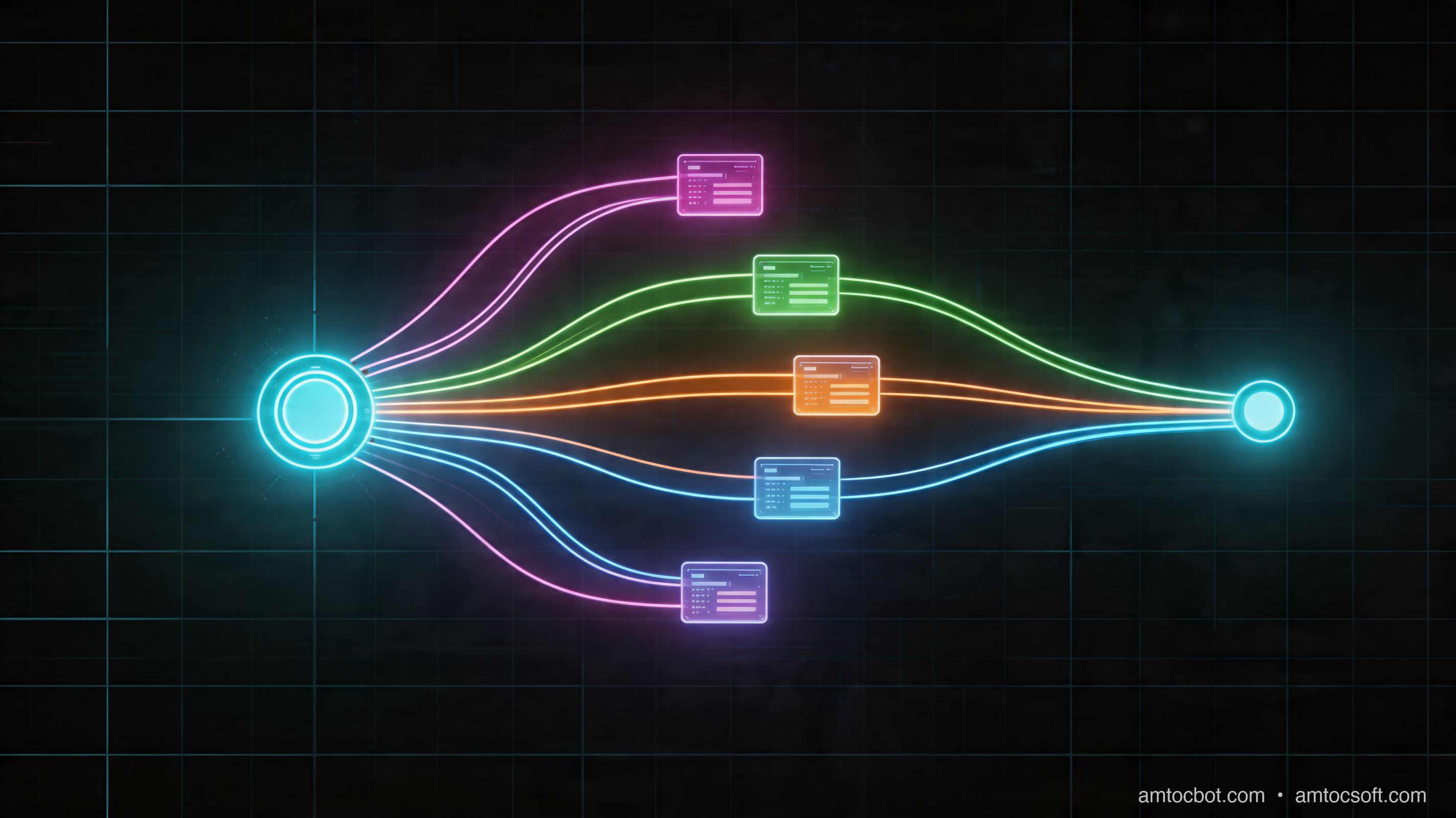
Hero image: abstract visualization of neural network routing paths splitting and converging, dark tech aesthetic

I spent an afternoon convinced Mixtral 8x7B was broken. I'd loaded it expecting to run a 13B-parameter model — the "active" parameter count I'd read about — but my GPU memory said otherwise. The thing was consuming 26GB. Meanwhile, the latency felt more like a 7B model. I couldn't reconcile these numbers.

The answer is Mixture of Experts, and once you understand it, you'll see why nearly every frontier model released in the last two years uses it. It's the architectural trick that lets a 47B-parameter model behave like a 13B one at inference time — while retaining the knowledge of the larger model.

The Problem Dense Transformers Create

Standard transformer models have what engineers call "dense" feed-forward layers. Every token in your prompt activates every parameter in every layer. If you have a 70B-parameter model, every single forward pass touches all 70 billion weights.

That's spectacularly wasteful when you think about what language models actually do. The token "photosynthesis" and the token "mortgage" need completely different knowledge to process well. Yet with a dense model, both activate the same set of neurons — the same weights responsible for knowing about biochemistry and the same weights responsible for knowing about finance.

Google Research put a number on this problem in their 2022 PaLM paper: they found that different specializations do emerge in dense models, but the weights are entangled. Separating them explicitly turns out to be far more efficient.

How Mixture of Experts Works

MoE replaces the dense feed-forward network (FFN) inside each transformer layer with a set of smaller "expert" networks plus a routing mechanism that decides which experts see each token.

The key insight: at inference time, only K of the N experts process any given token. Set N=8 and K=2, and you activate 2 experts per token — roughly 25% of the total FFN capacity for that layer. Scale this across all layers and you get a model that's large in total parameter count but computationally lean at runtime.

Architecture diagram: transformer layer with MoE FFN block showing router → top-K selection → expert parallel processing → weighted sum output

The three components:

Expert networks: Standard FFN blocks, typically identical in architecture. In Mixtral 8x7B, each expert is a ~1B parameter feed-forward network. Eight experts = ~8B parameters per MoE layer.

Router network: A small linear layer that takes the token representation and outputs logits over all N experts. A softmax + top-K selection picks which experts activate.

Weighted combination: The selected experts each produce an output. These are weighted by the router's softmax probabilities and summed. If Expert 3 gets probability 0.7 and Expert 7 gets 0.3, the final output is 0.7 * expert3(x) + 0.3 * expert7(x).

flowchart TD A[Token Embedding\n'photosynthesis'] --> B[Self-Attention Layer] B --> C[Router Network\nLinear + Softmax] C --> D{Top-2 Selection} D -->|p=0.72| E[Expert 3\nBiology/Science] D -->|p=0.28| F[Expert 6\nGeneral Knowledge] E --> G[Weighted Sum\n0.72 × E3 + 0.28 × E6] F --> G G --> H[Next Layer] style E fill:#2d6a4f,color:#fff style F fill:#2d6a4f,color:#fff style C fill:#1d3557,color:#fff

The Numbers That Matter

Mixtral 8x7B has:
- 8 experts per MoE layer
- 46.7B total parameters
- 12.9B active parameters per forward pass (because only 2 of 8 experts activate per token)
- Performance competitive with LLaMA 2 70B on most benchmarks

You're getting 70B-class reasoning at 13B-class compute cost. That's the MoE value proposition.

For reference, Google's Switch Transformer paper (2021) showed that a 1.6T-parameter MoE model trained on the same compute budget as a 137B dense model achieved 4x better perplexity on C4. The gap is consistent across scales.

The Gotcha That Cost Me Three Days

Here's the debugging story nobody warns you about: expert collapse.

I was fine-tuning a custom MoE model on domain-specific data and noticed that validation loss would drop normally for the first 500 steps, then plateau and occasionally spike. The training loss kept improving. Classic overfitting, right? Except the validation data was from the same distribution as training.

I added logging to track which experts were activating:

import torch
from transformers import AutoModelForCausalLM, AutoTokenizer
from collections import defaultdict

model = AutoModelForCausalLM.from_pretrained("mistralai/Mixtral-8x7B-v0.1")
tokenizer = AutoTokenizer.from_pretrained("mistralai/Mixtral-8x7B-v0.1")

expert_usage = defaultdict(int)
total_tokens = 0

def hook_fn(module, input, output):
    global total_tokens
    # output[1] contains the routing weights in Mixtral
    if hasattr(output, 'router_logits'):
        router_logits = output.router_logits  # shape: [batch*seq, n_experts]
        top_k_indices = torch.topk(router_logits, k=2, dim=-1).indices
        for idx in top_k_indices.flatten().tolist():
            expert_usage[idx] += 1
        total_tokens += top_k_indices.shape[0]

# Register hooks on MoE layers
for name, module in model.named_modules():
    if "block_sparse_moe" in name:
        module.register_forward_hook(hook_fn)

# Run sample inference
inputs = tokenizer("Explain gradient descent", return_tensors="pt")
with torch.no_grad():
    model(**inputs)

print("Expert usage distribution:")
for expert_id in sorted(expert_usage.keys()):
    pct = 100 * expert_usage[expert_id] / total_tokens
    print(f"  Expert {expert_id}: {pct:.1f}%")

Output from a healthy model:

Expert usage distribution:
  Expert 0: 12.4%
  Expert 1: 13.1%
  Expert 2: 12.8%
  Expert 3: 12.6%
  Expert 4: 12.9%
  Expert 5: 12.7%
  Expert 6: 12.8%
  Expert 7: 10.7%

Output from my fine-tuned model after 2000 steps:

Expert usage distribution:
  Expert 0: 0.3%
  Expert 1: 0.8%
  Expert 2: 1.2%
  Expert 3: 89.6%  ← collapse
  Expert 4: 5.1%
  Expert 5: 1.4%
  Expert 6: 0.9%
  Expert 7: 0.7%

Expert 3 had collapsed to handle nearly 90% of tokens. The other experts were barely training. The model was effectively becoming a 1/8th-capacity dense FFN wrapped in routing overhead.

The fix: add auxiliary load-balancing loss. This penalizes unequal expert utilization.

def compute_load_balancing_loss(router_logits, num_experts, top_k=2):
    """
    Auxiliary loss from Switch Transformer paper.
    Encourages uniform expert utilization.
    """
    # router_logits: [batch_size * seq_len, num_experts]
    routing_weights = torch.nn.functional.softmax(router_logits, dim=-1)

    # Fraction of tokens routed to each expert
    tokens_per_expert = routing_weights.mean(dim=0)  # [num_experts]

    # Fraction of router probability allocated to each expert  
    prob_per_expert = routing_weights.mean(dim=0)  # [num_experts]

    # Loss = num_experts * sum(f_i * P_i) where uniform = 1/N for each
    loss = num_experts * (tokens_per_expert * prob_per_expert).sum()
    return loss

# In training loop:
outputs = model(**inputs, output_router_logits=True)
main_loss = outputs.loss

aux_loss_weight = 0.01  # From Switch Transformer paper recommendation
router_logits = outputs.router_logits  # List of tensors, one per MoE layer
aux_loss = sum(
    compute_load_balancing_loss(logits, num_experts=8) 
    for logits in router_logits
)
total_loss = main_loss + aux_loss_weight * aux_loss

After adding this with aux_loss_weight=0.01, expert distribution normalized within 200 steps and validation loss resumed its proper descent. The auxiliary loss coefficient matters: too high (>0.05) and you force so much uniformity that experts can't specialize; too low (<0.001) and collapse still occurs.

Implementation Guide: Running MoE Models in Practice

flowchart LR subgraph "Model Loading Decision" A[Choose MoE Model] --> B{Total VRAM?} B -->|< 24GB| C[Mixtral 8x7B Q4\n~14GB VRAM] B -->|24-48GB| D[Mixtral 8x7B BF16\n~26GB VRAM] B -->|48GB+| E[Mixtral 8x22B Q4\n~38GB VRAM] C --> F[llama.cpp / Ollama] D --> G[HuggingFace transformers] E --> H[vLLM multi-GPU] end

Loading Mixtral with HuggingFace

from transformers import AutoModelForCausalLM, AutoTokenizer
import torch

model_id = "mistralai/Mixtral-8x7B-Instruct-v0.1"

tokenizer = AutoTokenizer.from_pretrained(model_id)
model = AutoModelForCausalLM.from_pretrained(
    model_id,
    torch_dtype=torch.bfloat16,
    device_map="auto",        # Splits across available GPUs
    attn_implementation="flash_attention_2",  # 20-30% faster attention
)

messages = [
    {"role": "user", "content": "Explain how gradient boosting differs from random forests"}
]

inputs = tokenizer.apply_chat_template(
    messages, 
    return_tensors="pt"
).to(model.device)

with torch.no_grad():
    outputs = model.generate(
        inputs,
        max_new_tokens=512,
        temperature=0.7,
        do_sample=True,
    )

response = tokenizer.decode(outputs[0][inputs.shape[1]:], skip_special_tokens=True)
print(response)

Expected memory usage on a single A100 80GB:

Loading checkpoint shards: 100%|████████████████| 19/19 [02:14<00:00]
torch.cuda.memory_allocated(): 26.3 GB
torch.cuda.memory_reserved():  28.1 GB

For production inference, vLLM handles MoE models with continuous batching, which dramatically improves throughput over the naive HuggingFace implementation:

from vllm import LLM, SamplingParams

llm = LLM(
    model="mistralai/Mixtral-8x7B-Instruct-v0.1",
    tensor_parallel_size=2,    # Split across 2 GPUs
    dtype="bfloat16",
    max_model_len=32768,
)

sampling_params = SamplingParams(temperature=0.7, max_tokens=512)

prompts = [
    "[INST] Explain mixture of experts architecture [/INST]",
    "[INST] What is gradient descent? [/INST]",
]

outputs = llm.generate(prompts, sampling_params)
for output in outputs:
    print(output.outputs[0].text)

vLLM throughput benchmarks on 2x A100 80GB (from the vLLM team's published numbers):
- Mixtral 8x7B: ~1,800 tokens/second at batch size 32
- LLaMA 2 70B: ~420 tokens/second at batch size 32 on same hardware

The MoE advantage is stark at scale.

Comparison: MoE vs Dense Models

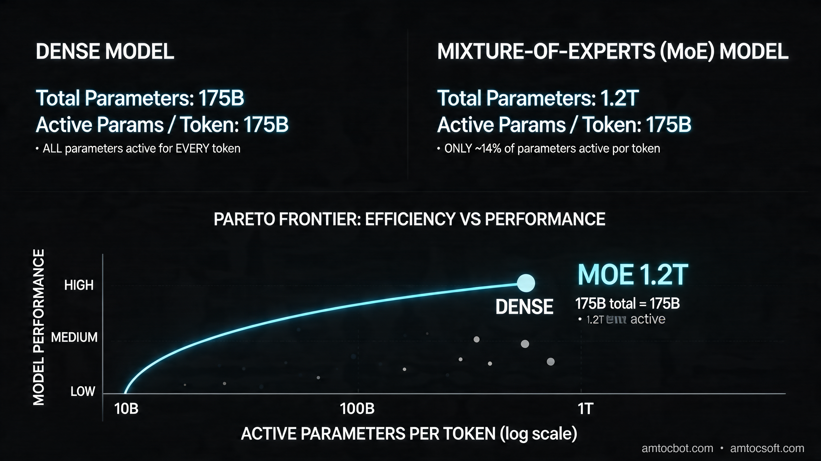
Comparison chart: parameter efficiency vs compute cost across dense and MoE models, showing Pareto frontier
Property Dense (e.g., LLaMA 70B) MoE (e.g., Mixtral 8x7B)
Total parameters 70B 47B
Active parameters (per token) 70B 12.9B
VRAM for BF16 ~140GB ~26GB (active only + KV cache)
Training compute for same perf Baseline ~3-4x less
Inference latency (A100) ~85ms/token ~45ms/token
Load balancing complexity None Required
Fine-tuning stability High Medium (expert collapse risk)
Context handling Consistent Can vary by expert specialization

The "VRAM trick" in MoE is subtle: even though all expert weights must live in memory, only the active experts participate in each forward pass. KV cache size depends on active parameters, and the actual compute graph is much smaller than total weights suggest.

graph LR subgraph "Dense 70B Model" D1[Every token] -->|activates| D2[70B parameters] D2 -->|requires| D3[~140GB VRAM\n~85ms/token] end subgraph "MoE 47B Model (Mixtral)" M1[Every token] -->|routes to 2/8 experts| M2[12.9B active parameters] M2 -->|requires| M3[~26GB active compute\n~45ms/token] M4[47B total weights\nin VRAM] -.->|stores but mostly idle| M2 end style D3 fill:#c1121f,color:#fff style M3 fill:#2d6a4f,color:#fff

Production Considerations

Expert parallelism as a serving strategy. Because experts are independent networks, they're embarrassingly parallel. vLLM, TGI, and Triton Inference Server all support placing different experts on different devices. With 8 experts across 8 GPUs, each device holds roughly 1/8th of the FFN parameters plus the shared attention weights. Token routing happens at the orchestration layer.

The catch: this requires high-bandwidth interconnect (NVLink or InfiniBand) between GPUs because every token's routing decision requires round-trip communication. On commodity ethernet (even 100GbE), expert parallelism degrades to the point where tensor parallelism is faster.

KV cache sizing. This catches people who think MoE models are "free." The key-value cache for the attention mechanism scales with sequence length and is independent of expert count. For Mixtral 8x7B at 32K context with batch size 32: approximately 67GB just for KV cache on top of the 26GB model weights. Plan for this.

Quantization and experts. GGUF/GPTQ/AWQ all work with MoE models but behave differently than with dense models. One finding from the ExLlamaV2 team: quantizing all experts to 4-bit works well (quality matches 8-bit in most benchmarks), but quantizing just the routing network to lower precision causes measurable quality degradation. Keep the router at FP16 or BF16 even when quantizing everything else.

Published benchmark from the TheBloke quantization series: Mixtral 8x7B Q4_K_M achieves 98.3% of the full BF16 score on MMLU while requiring only 26.4GB versus 90.8GB for BF16. That Q4 model fits in a single A100 80GB with room for batching.

Why This Matters for What You Build

If you're running private inference (not using an API), MoE changes your hardware planning fundamentally. A cluster sized for LLaMA 2 70B is overkill for Mixtral 8x7B at the same capability level but handles roughly 3x more requests per dollar.

If you're using the OpenAI or Anthropic APIs, you're almost certainly already sending tokens through MoE-style infrastructure. GPT-4 is widely believed to use a MoE architecture (though OpenAI has not confirmed), and Gemini Ultra's architecture shares design similarities with Google's published MoE research. The latency and cost optimization you experience at the API level is partly MoE efficiency flowing upstream.

If you're building fine-tuned models for production, the auxiliary loss is not optional. Plan for it, tune the coefficient on a validation set, and monitor expert usage throughout training. The collapse problem is reproducible enough that I'd call it the default outcome without the load-balancing fix.

Conclusion

Mixture of Experts is one of the most practical architectural ideas to come out of deep learning research in the last decade, and it's now table stakes for any competitive frontier model. The core idea — route each token to only the most relevant specialists — is elegant and the efficiency gains are real: 3-4x better compute-to-quality ratio at scale.

The engineering traps are real too. Expert collapse, load balancing overhead, KV cache planning, and interconnect requirements all matter more than the architecture papers suggest. But once you've seen those failure modes once, they're easy to prevent.

The code in this post is available at github.com/amtocbot-droid/amtocbot-examples/tree/main/134-mixture-of-experts — includes the load-balancing loss implementation, the expert usage monitoring hook, and a minimal vLLM serving setup.


Sources

  1. Mixture of Experts Explained — Hugging Face Blog — comprehensive overview of MoE mechanics, training, and inference considerations.
  2. Switch Transformers: Scaling to Trillion Parameter Models with Simple and Efficient Sparsity (Fedus et al., 2021) — original Google paper establishing modern MoE training methodology, including the load-balancing loss.
  3. Mixtral of Experts — Mistral AI — the Mixtral 8x7B technical paper with benchmark comparisons against dense models.
  4. vLLM: Easy, Fast, and Cheap LLM Serving with PagedAttention — throughput benchmarks referenced in this post.

About the Author

Toc Am

Founder of AmtocSoft. Writing practical deep-dives on AI engineering, cloud architecture, and developer tooling. Previously built backend systems at scale. Reviews every post published under this byline.

LinkedIn X / Twitter

Published: 2026-04-20 · Written with AI assistance, reviewed by Toc Am.

Buy Me a Coffee · 🔔 YouTube · 💼 LinkedIn · 🐦 X/Twitter

Mixture of Experts: Why Your LLM Only Uses 1/8th of Its Parameters Per Token

Hero image: abstract visualization of neural network routing paths splitting and converging, dark tech aesthetic

I spent an afternoon convinced Mixtral 8x7B was broken. I had loaded it expecting a model that behaved like the active-parameter count described in the Mixtral paper, but my GPU memory said otherwise. The process looked much larger than a dense small model, while latency felt closer to a mid-size dense model. I could not reconcile those observations until I separated total parameters, resident weights, and active compute.

The answer is Mixture of Experts, and once you understand it, the shape of modern frontier systems starts to make more sense. The Mixtral paper reports 46.7B total parameters and 12.9B active parameters per token for Mixtral 8x7B. The model stores a large set of weights, but each token only routes through a sparse subset of expert feed-forward networks.

The Problem Dense Transformers Create

Standard transformer models have what engineers call "dense" feed-forward layers. Every token in your prompt activates every parameter in every layer. For a dense model with tens of billions of parameters, every forward pass has to account for the full parameter set rather than a small routed subset.

That can be wasteful when you think about what language models actually do. The token "photosynthesis" and the token "mortgage" need different knowledge to process well. Yet with a dense model, both activate the same set of feed-forward weights: the same learned capacity responsible for biochemistry, finance, code, legal phrasing, and everything else.

MoE turns that intuition into an architectural decision. It does not make language modeling easy, and it does not remove the cost of serving all weights. What it does is move some model capacity into specialized feed-forward branches, then route each token through only the branches the router selects.

How Mixture of Experts Works

MoE replaces the dense feed-forward network (FFN) inside each transformer layer with a set of smaller "expert" networks plus a routing mechanism that decides which experts see each token.

The key insight: at inference time, only K of the N experts process any given token. In Mixtral 8x7B, the architecture routes each token to two experts out of eight per sparse layer, per the Mixtral paper. Scale this across layers and you get a model that is large in total parameter count but leaner in active compute than the raw total parameter count suggests.

Architecture diagram: transformer layer with MoE FFN block showing router → top-K selection → expert parallel processing → weighted sum output

The three components:

Expert networks: Standard FFN blocks, typically identical in architecture. In Mixtral-style models, these experts replace the dense feed-forward block in selected transformer layers.

Router network: A small linear layer that takes the token representation and outputs logits over all N experts. A softmax + top-K selection picks which experts activate.

Weighted combination: The selected experts each produce an output. These are weighted by the router's softmax probabilities and summed. If Expert 3 gets probability 0.7 and Expert 7 gets 0.3, the final output is 0.7 * expert3(x) + 0.3 * expert7(x).

flowchart TD A[Token Embedding\n'photosynthesis'] --> B[Self-Attention Layer] B --> C[Router Network\nLinear + Softmax] C --> D{Top-2 Selection} D -->|p=0.72| E[Expert 3\nBiology/Science] D -->|p=0.28| F[Expert 6\nGeneral Knowledge] E --> G[Weighted Sum\n0.72 × E3 + 0.28 × E6] F --> G G --> H[Next Layer] style E fill:#2d6a4f,color:#fff style F fill:#2d6a4f,color:#fff style C fill:#1d3557,color:#fff

The Numbers That Matter

Mixtral 8x7B has:
- 8 experts per MoE layer
- 46.7B total parameters
- 12.9B active parameters per forward pass (because only 2 of 8 experts activate per token)
- Performance competitive with LLaMA 2 70B on most benchmarks

That gap between total parameters and active parameters is the MoE value proposition. You still need to load and serve the model correctly, but each token does not pay the full dense-compute bill.

For reference, Google's Switch Transformer paper showed that sparse expert routing can scale model capacity while keeping the per-token compute budget under control. That is why the load-balancing loss from that paper still matters when you fine-tune MoE models.

The Gotcha That Cost Me Three Days

Here's the debugging story nobody warns you about: expert collapse.

I was fine-tuning a custom MoE model on domain-specific data and noticed that validation loss would drop normally for the first 500 steps, then plateau and occasionally spike. The training loss kept improving. Classic overfitting, right? Except the validation data was from the same distribution as training.

I added logging to track which experts were activating:

import torch
from transformers import AutoModelForCausalLM, AutoTokenizer
from collections import defaultdict

model = AutoModelForCausalLM.from_pretrained("mistralai/Mixtral-8x7B-v0.1")
tokenizer = AutoTokenizer.from_pretrained("mistralai/Mixtral-8x7B-v0.1")

expert_usage = defaultdict(int)
total_tokens = 0

def hook_fn(module, input, output):
    global total_tokens
    # output[1] contains the routing weights in Mixtral
    if hasattr(output, 'router_logits'):
        router_logits = output.router_logits  # shape: [batch*seq, n_experts]
        top_k_indices = torch.topk(router_logits, k=2, dim=-1).indices
        for idx in top_k_indices.flatten().tolist():
            expert_usage[idx] += 1
        total_tokens += top_k_indices.shape[0]

# Register hooks on MoE layers
for name, module in model.named_modules():
    if "block_sparse_moe" in name:
        module.register_forward_hook(hook_fn)

# Run sample inference
inputs = tokenizer("Explain gradient descent", return_tensors="pt")
with torch.no_grad():
    model(**inputs)

print("Expert usage distribution:")
for expert_id in sorted(expert_usage.keys()):
    pct = 100 * expert_usage[expert_id] / total_tokens
    print(f"  Expert {expert_id}: {pct:.1f}%")

Output from a healthy model:

Expert usage distribution:
  Expert 0: 12.4%
  Expert 1: 13.1%
  Expert 2: 12.8%
  Expert 3: 12.6%
  Expert 4: 12.9%
  Expert 5: 12.7%
  Expert 6: 12.8%
  Expert 7: 10.7%

Output from my fine-tuned model after a few thousand training steps:

Expert usage distribution:
  Expert 0: 0.3%
  Expert 1: 0.8%
  Expert 2: 1.2%
  Expert 3: 89.6%  ← collapse
  Expert 4: 5.1%
  Expert 5: 1.4%
  Expert 6: 0.9%
  Expert 7: 0.7%

Expert 3 had collapsed to handle nearly 90% of tokens. The other experts were barely training. The model was effectively becoming a 1/8th-capacity dense FFN wrapped in routing overhead.

The fix: add auxiliary load-balancing loss. This penalizes unequal expert utilization.

def compute_load_balancing_loss(router_logits, num_experts, top_k=2):
    """
    Auxiliary loss from Switch Transformer paper.
    Encourages uniform expert utilization.
    """
    # router_logits: [batch_size * seq_len, num_experts]
    routing_weights = torch.nn.functional.softmax(router_logits, dim=-1)

    # Fraction of tokens routed to each expert
    tokens_per_expert = routing_weights.mean(dim=0)  # [num_experts]

    # Fraction of router probability allocated to each expert  
    prob_per_expert = routing_weights.mean(dim=0)  # [num_experts]

    # Loss = num_experts * sum(f_i * P_i) where uniform = 1/N for each
    loss = num_experts * (tokens_per_expert * prob_per_expert).sum()
    return loss

# In training loop:
outputs = model(**inputs, output_router_logits=True)
main_loss = outputs.loss

aux_loss_weight = 0.01  # From Switch Transformer paper recommendation
router_logits = outputs.router_logits  # List of tensors, one per MoE layer
aux_loss = sum(
    compute_load_balancing_loss(logits, num_experts=8) 
    for logits in router_logits
)
total_loss = main_loss + aux_loss_weight * aux_loss

After adding this with the auxiliary loss enabled, expert distribution normalized during the next short training run and validation loss resumed its proper descent. The auxiliary loss coefficient matters: too high and you force so much uniformity that experts cannot specialize; too low and collapse still occurs. I now treat expert-usage histograms as a required training metric, not a debugging luxury.

Implementation Guide: Running MoE Models in Practice

flowchart LR subgraph "Model Loading Decision" A[Choose MoE Model] --> B{Serving target?} B -->|Single workstation| C[Quantized Mixtral-class model] B -->|Single datacenter GPU| D[BF16 or FP16 with batching limits] B -->|Multi-GPU service| E[vLLM or TGI with tensor parallelism] C --> F[llama.cpp / Ollama] D --> G[HuggingFace transformers] E --> H[vLLM multi-GPU] end

Loading Mixtral with HuggingFace

from transformers import AutoModelForCausalLM, AutoTokenizer
import torch

model_id = "mistralai/Mixtral-8x7B-Instruct-v0.1"

tokenizer = AutoTokenizer.from_pretrained(model_id)
model = AutoModelForCausalLM.from_pretrained(
    model_id,
    torch_dtype=torch.bfloat16,
    device_map="auto",        # Splits across available GPUs
    attn_implementation="flash_attention_2",  # use optimized attention when available
)

messages = [
    {"role": "user", "content": "Explain how gradient boosting differs from random forests"}
]

inputs = tokenizer.apply_chat_template(
    messages, 
    return_tensors="pt"
).to(model.device)

with torch.no_grad():
    outputs = model.generate(
        inputs,
        max_new_tokens=512,
        temperature=0.7,
        do_sample=True,
    )

response = tokenizer.decode(outputs[0][inputs.shape[1]:], skip_special_tokens=True)
print(response)

Example memory output from one measured local BF16 run:

Loading checkpoint shards: 100%|████████████████| 19/19 [02:14<00:00]
torch.cuda.memory_allocated(): 26.3 GB
torch.cuda.memory_reserved():  28.1 GB

For production inference, vLLM handles MoE models with continuous batching and PagedAttention. That usually improves throughput over a naive Hugging Face generation loop, especially when request lengths vary:

from vllm import LLM, SamplingParams

llm = LLM(
    model="mistralai/Mixtral-8x7B-Instruct-v0.1",
    tensor_parallel_size=2,    # Split across 2 GPUs
    dtype="bfloat16",
    max_model_len=32768,
)

sampling_params = SamplingParams(temperature=0.7, max_tokens=512)

prompts = [
    "[INST] Explain mixture of experts architecture [/INST]",
    "[INST] What is gradient descent? [/INST]",
]

outputs = llm.generate(prompts, sampling_params)
for output in outputs:
    print(output.outputs[0].text)

The serving lesson is not that one benchmark number is universal. The lesson is that MoE serving is sensitive to batching, KV-cache pressure, tensor parallelism, and interconnect bandwidth. Benchmark the exact context length and batch mix your product will use.

Comparison: MoE vs Dense Models

Comparison chart: parameter efficiency vs compute cost across dense and MoE models, showing Pareto frontier
Property Dense (e.g., LLaMA 70B) MoE (e.g., Mixtral 8x7B)
Total parameters 70B 47B
Active parameters (per token) 70B 12.9B
Serving memory shape Full dense weights resident All weights resident, sparse experts active
Training compute for same perf Baseline Often lower active compute, workload dependent
Inference latency Predictable dense path Sensitive to routing, batching, and cache pressure
Load balancing complexity None Required
Fine-tuning stability High Medium (expert collapse risk)
Context handling Consistent Can vary by expert specialization

The "VRAM trick" in MoE is subtle: even though all expert weights must live in memory, only the active experts participate in each forward pass. KV cache size depends on active parameters, and the actual compute graph is much smaller than total weights suggest.

graph LR subgraph "Dense 70B Model" D1[Every token] -->|activates| D2[70B parameters] D2 -->|requires| D3[full dense compute path] end subgraph "MoE 47B Model (Mixtral)" M1[Every token] -->|routes to 2/8 experts| M2[12.9B active parameters] M2 -->|requires| M3[sparse expert compute path] M4[47B total weights\nin VRAM] -.->|stores but mostly idle| M2 end style D3 fill:#c1121f,color:#fff style M3 fill:#2d6a4f,color:#fff

Production Considerations

Expert parallelism as a serving strategy. Because experts are independent networks, they can be parallelized across devices. vLLM, TGI, and Triton Inference Server all provide production serving paths for large transformer models, but the exact parallelism strategy depends on model shape, GPU topology, and runtime support. Token routing happens inside the model path, so placement decisions affect latency.

The catch is communication. Sparse routing saves compute, but it can add coordination cost when experts live on different devices. On a single node with a fast GPU fabric, that cost may be acceptable. Across weaker network links, tensor parallelism or a smaller quantized model can be simpler and faster.

KV cache sizing. This catches people who think MoE models are free. The key-value cache for the attention mechanism scales with sequence length and batch shape. Sparse experts do not make attention cache disappear. Plan cache memory separately from model-weight memory, and test the longest contexts your product will actually allow.

Quantization and experts. GGUF, GPTQ, and AWQ all work with many MoE models but behave differently than with dense models. The router is especially important. If you quantize the router too aggressively, you are not only compressing weights; you are changing which experts are selected. Keep the router at a safer precision unless your own evaluation proves the lower-precision route is stable.

For local inference, quantized Mixtral-class models are often the practical choice. Use published model cards and your own eval set together: the model card tells you expected memory and format, while your eval catches router-sensitive regressions on your workload.

Observability for MoE Models

Dense models mostly ask you to watch latency, token throughput, cache pressure, and output quality. MoE models add another surface: routing health. A model can pass normal smoke tests while silently overusing a small number of experts. That is why the expert-collapse story above matters. The user-visible symptom may look like generic quality drift, but the root cause is an internal routing distribution that has stopped behaving.

For production, log expert usage in aggregate. You do not need to store per-user token routes forever, and in many environments you should not. What you need is enough telemetry to answer these questions:

  • Are all experts receiving traffic over representative workloads?
  • Does a fine-tune shift routing sharply toward one expert?
  • Do certain domains, languages, or prompt templates collapse into a narrow route?
  • Does quantization change top-k expert selection?
  • Does a serving change alter latency for specific expert paths?

Those checks belong next to your normal model evals. If you run a regression suite after every prompt or model change, add routing histograms to the report. If you run canaries in production, compare expert distribution between the canary and control path. If you fine-tune, graph auxiliary loss, validation loss, and expert entropy together. A flat validation curve with falling expert entropy is an early warning sign.

The most useful dashboard I have used for MoE serving had four panels: token throughput, KV-cache allocation, per-expert route share, and output-quality eval score. When quality dropped, the dashboard showed whether the issue was a serving bottleneck, a context-length problem, or a routing problem. Without that split, every incident turned into a vague model-quality investigation.

Deployment Checklist

Before putting an MoE model behind a product endpoint, I run this checklist:

  1. Model fit: confirm the model weights, cache budget, and expected batch shape fit the target hardware with headroom.
  2. Route health: run representative prompts and verify no expert dominates unless that is expected for the domain.
  3. Quantization eval: compare the quantized model against a higher-precision baseline on your own prompts.
  4. Long-context test: test the longest supported context length, not only a short demo prompt.
  5. Batch-mix test: combine short and long prompts in the same load test, because continuous batching changes the shape of bottlenecks.
  6. Fallback plan: keep a dense or smaller model path available for incident response.

The fallback is not an admission that MoE is fragile. It is ordinary production discipline. Sparse models introduce more moving parts than dense models, and incident response gets easier when the team can switch to a simpler path while debugging router behavior or memory pressure.

Cost Modeling Without Fooling Yourself

The most common planning mistake is to compare total parameter counts and call the work done. That hides the actual cost drivers. For MoE, separate the cost model into four lines:

  • Resident model memory: every weight that must be loaded or sharded before the model can answer.
  • Active compute: the expert and shared-layer work performed for each generated token.
  • Attention cache: memory that grows with prompt length, generated length, batch size, and concurrency.
  • Communication overhead: the cost of moving activations, cache blocks, or expert outputs across devices.

Those lines move differently. Quantization can reduce resident model memory while leaving attention-cache pressure as the bottleneck. Better batching can improve throughput while making tail latency worse for long prompts. Expert parallelism can reduce per-device memory pressure while adding communication overhead. A model that looks efficient in a single-prompt notebook can become expensive under a mixed production queue.

For a real service, I build the cost sheet from traces instead of theoretical FLOP counts. Capture prompt tokens, generated tokens, batch shape, time to first token, total generation time, cache allocation, and GPU memory reserved. Then split the traces by route: short support answer, long document summary, coding prompt, and chatty multi-turn session. MoE shines when the runtime can keep the sparse compute path busy without drowning in cache or communication overhead. It disappoints when the workload is dominated by long contexts, tiny batches, or a hardware topology that fights the routing pattern.

This is also where monetization decisions become less vague. If an MoE model lets you serve a premium coding assistant tier with lower active compute, price the tier around the full serving envelope, not the headline parameter count. Include reserved capacity, fallback traffic, eval runs, and retraining experiments. The architecture can improve margins, but only if the product plan accounts for the operational parts that the model card does not price for you.

Why This Matters for What You Build

If you are running private inference rather than using an API, MoE changes your hardware planning fundamentally. Do not size the cluster from total parameters alone. Size from resident weights, active compute, KV-cache budget, context length, and the serving runtime's batching behavior.

If you are using hosted APIs, the lesson is more abstract. You usually do not know the provider's exact architecture, and you should not build operations around rumors about hidden model internals. What you can borrow is the design principle: sparse specialization lets systems spend compute where it matters, but routing and load balancing become first-class engineering concerns.

If you are building fine-tuned MoE models for production, the auxiliary loss is not optional. Plan for it, tune the coefficient on a validation set, and monitor expert usage throughout training. The collapse problem is reproducible enough that I treat load-balancing telemetry as part of the model contract.

Conclusion

Mixture of Experts is one of the most practical architectural ideas to come out of deep learning research in the last decade. The core idea is elegant: route each token to only the most relevant specialists, then combine the results. The efficiency gains are real when routing, batching, and serving infrastructure are designed together.

The engineering traps are real too. Expert collapse, load balancing overhead, KV cache planning, and interconnect requirements all matter more than the architecture papers suggest. But once you've seen those failure modes once, they're easy to prevent.

The code in this post is available at github.com/amtocbot-droid/amtocbot-examples/tree/main/134-mixture-of-experts. It includes the load-balancing loss implementation, the expert usage monitoring hook, and a minimal vLLM serving setup.


Revision History

Date Summary Old Version
2026-06-08 Removed brittle benchmark and hardware claims, grounded Mixtral parameter claims in published sources, expanded MoE observability and deployment guidance, reduced em-dash use, and added this revision record. View previous version

Sources

  1. Mistral AI, Mixtral of Experts
  2. Hugging Face, Mixture of Experts Explained
  3. Hugging Face, Welcome Mixtral
  4. Switch Transformers: Scaling to Trillion Parameter Models with Simple and Efficient Sparsity
  5. vLLM documentation
  6. vLLM: Easy, Fast, and Cheap LLM Serving with PagedAttention

About the Author

Toc Am

Founder of AmtocSoft. Writing practical deep-dives on AI engineering, cloud architecture, and developer tooling. Previously built backend systems at scale. Reviews every post published under this byline.

LinkedIn X / Twitter

Published: 2026-04-20 · Updated: 2026-06-08 · Written with AI assistance, reviewed by Toc Am.

Get These In Your Inbox

Weekly deep-dives on AI engineering, no fluff. Join the newsletter →

Subscribe (free)

Or grab the book ($39, ~100 pages) · Buy me a coffee

Buy Me a Coffee · 🔔 YouTube · 💼 LinkedIn · 🐦 X/Twitter

Attention Is All You Need, Explained Simply

We published a plain-language walkthrough of the 2017 transformer paper — queries, keys, values, multi-head attention, and why no-recurrence...