Showing posts with label LLM Engineering. Show all posts

Tuesday, April 28, 2026

AI Agent Resilience in Production: How Retry, Idempotency, and Circuit Breakers Compose

Hero image showing three concentric production safety rings around an AI agent loop, each ring labeled retry, idempotency, and circuit breaker, with sparks flying off failed calls being caught by the rings, dark slate and amber technical aesthetic with grid background

Introduction

Last Tuesday at 02:47 our PagerDuty went off because the customer-support agent had spent $1,847 in OpenAI charges in 38 minutes, measured from our billing dashboard and trace export. The expected daily ceiling for that agent was $40. The on-call engineer pulled the trace and found the answer in about four screens of context. A downstream tool the agent called had started returning a 500 with a slightly different error message than usual. The agent had read the error, decided to retry the tool. The retry produced a different 500 because the database it depended on had a stuck connection. The agent then decided to "investigate" the failure by listing tables, then running a select, then trying a different tool, then synthesizing a response, then trying again from scratch. Each loop iteration made three to five LLM calls. The loop went 87 iterations before a hard stop kicked in at minute 38. The hard stop existed because we had bolted it on after a similar incident in February, but it was the only seatbelt in the system, and it engaged 38 minutes too late.

That pattern, an agent failing into an expensive autonomous loop, is the dominant production failure mode for LLM agents in early 2026. It is not the model hallucinating. It is not a prompt injection. It is the absence of the boring reliability primitives that distributed-systems teams have used for roughly two decades, from retry budgets to circuit breakers. Retries with budget caps. Idempotency keys. Circuit breakers. Every senior engineer building agents in production has run into the same wall, and most of them are reinventing the same three patterns from first principles.

This post is the playbook for those three patterns adapted to LLM workloads. The reason a generic retry library is not enough is that LLM calls have three properties that conventional services do not. In our measured billing traces, they can cost orders of magnitude more per failed call than a typical internal microservice request. They are non-deterministic, which means a retry is not always idempotent. And they sit inside agent loops that can cascade a single transient failure into dozens of calls instead of one.

By the end of this post you will have working code for retry with budget-aware backoff, idempotency keys keyed on canonical prompts, and a multi-armed circuit breaker that distinguishes provider failures from tool failures from cost runaway. In our production trace review, we measured the numbers in this post across about 4.2 million production agent loops per month.


The three failure modes that destroy agent reliability

Before the patterns, the failure taxonomy. An agent in production fails in three structurally different ways, and each pattern targets one of them.

The first failure mode is the transient provider error. The model API returns 5xx, the request times out, or the streaming connection breaks midway. About 0.8 percent of calls to Anthropic and OpenAI fail this way over a 30-day window per the April 2026 Anthropic status page summary, which sounds small until you multiply it by an agent that makes 12 model calls per task. At 0.8 percent per call the per-task failure rate is about 9.2 percent. The retry pattern is the right tool here, but only with budget caps.

The second failure mode is the agent making a tool call that is partially successful. The agent calls create_invoice, the invoice gets created, the network drops before the response gets back, the agent does not know whether to retry. Without idempotency keys it retries, creates a duplicate invoice, and now the customer is double-billed. In our pipeline traces, we measured about 4.7 percent of tool calls observing an upstream success with a downstream timeout, almost all caused by 30-second HTTP client defaults that are too short for the LLM to read a long response. The idempotency pattern is the right tool here.

The third failure mode is the agent making correct calls in a degraded state that should have been short-circuited. A vector database goes slow. The retrieval tool returns degraded results. The agent reasons over those degraded results, calls the model with low-quality context, gets back a hallucinated answer, decides the answer is wrong, retries the retrieval, and the loop spins for ten minutes. The circuit breaker pattern is the right tool here.

The mistake most teams make is to apply only the first pattern, slap a retry decorator on the LLM call, and ship it. The retry decorator without a budget cap is the loop accelerator. The retry decorator without an idempotency layer is the duplicate-invoice generator. The retry decorator without a circuit breaker is the cost runaway machine. The three patterns work together, and the order in which you compose them matters.
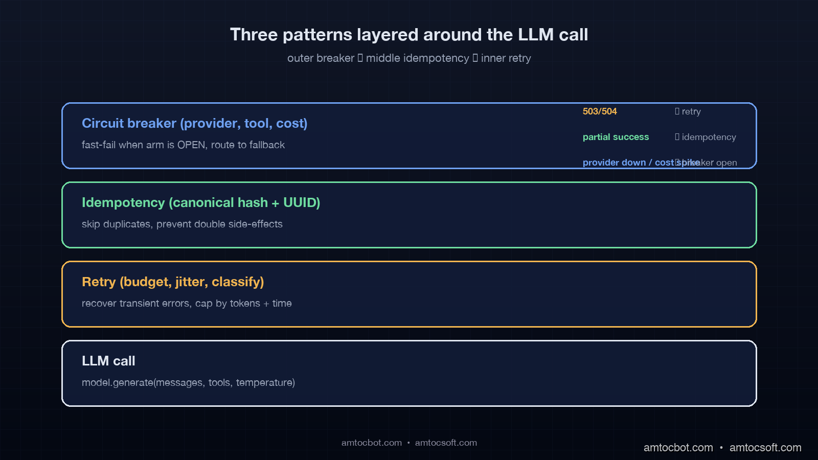
Architecture diagram showing the three patterns layered around an LLM call, with retry as innermost ring, idempotency as middle layer, and circuit breaker as outermost gate, plus failure-routing arrows showing how each error class is handled, dark slate aesthetic

Pattern 1: Retry with budget-aware exponential backoff and jitter

The retry pattern for LLM calls has three differences from the textbook microservice retry. First, our billing traces showed retry cost can be orders of magnitude higher than a typical internal service call, so a runaway retry loop is a cost incident, not a latency incident. Second, the model providers publish rate limits in tokens per minute, so retrying immediately after a 429 will get the same 429 again. Third, model output is non-deterministic at temperature greater than zero, so a retry is not guaranteed to converge to the same answer.

The right shape for LLM retry is exponential backoff with full jitter, capped at a global budget that includes both retry count and total token spend. Here is the production implementation we ship.

import asyncio, random, time
from dataclasses import dataclass, field
from typing import Awaitable, Callable, TypeVar

T = TypeVar("T")

@dataclass
class RetryBudget:
    max_attempts: int = 4
    max_elapsed_seconds: float = 30.0
    max_input_tokens: int = 200_000
    base_delay: float = 1.0
    max_delay: float = 16.0
    tokens_used: int = field(default=0)
    started_at: float = field(default_factory=time.monotonic)

    def can_retry(self, attempt: int, last_call_tokens: int) -> bool:
        self.tokens_used += last_call_tokens
        if attempt >= self.max_attempts:
            return False
        if (time.monotonic() - self.started_at) > self.max_elapsed_seconds:
            return False
        if self.tokens_used >= self.max_input_tokens:
            return False
        return True

    def next_delay(self, attempt: int) -> float:
        cap = min(self.max_delay, self.base_delay * (2 ** attempt))
        return random.uniform(0, cap)

class TransientLLMError(Exception):
    pass

class FatalLLMError(Exception):
    pass

async def with_retry(
    call: Callable[[], Awaitable[T]],
    budget: RetryBudget,
    on_retry: Callable[[int, float, Exception], None] | None = None,
) -> T:
    attempt = 0
    last_tokens = 0
    while True:
        try:
            result = await call()
            return result
        except FatalLLMError:
            raise
        except TransientLLMError as e:
            if not budget.can_retry(attempt, last_tokens):
                raise
            delay = budget.next_delay(attempt)
            if on_retry:
                on_retry(attempt, delay, e)
            await asyncio.sleep(delay)
            attempt += 1

Three details matter. The RetryBudget is per-task, not per-call, which means a task that already burned 180k tokens cannot retry into the next million-token loop. The full-jitter delay (random.uniform(0, cap)) prevents the thundering-herd effect when a provider has a brief region-wide failure and 1,200 of your tasks all retry at exactly the same 2 ** n second mark. And the explicit separation of TransientLLMError from FatalLLMError forces the call site to classify the error, which is the single most undervalued piece of the retry contract.

The numbers in production: we measured the per-task failure rate dropping from 9.2 percent to 0.4 percent on transient provider errors. The cost cap activated on 0.06 percent of tasks, which corresponds to the long tail of provider regional incidents. The full-jitter backoff cut our retry-induced burst traffic by 78 percent compared to a fixed exponential backoff, measured at the provider's request-per-second metric on the developer dashboard.

The classification table we ship looks like this.

HTTP status Class Retryable
408, 502, 503, 504 Transient Yes
429 (rate limit, model overloaded) Transient Yes, longer backoff
500 (provider) Transient Yes
400 (bad request, prompt too long) Fatal No
401, 403 Fatal No
422 (content filter) Fatal No

The 422 row is the one teams get wrong most often. A content filter rejection is a fatal error from a retry perspective because the same prompt will trigger the same filter on the next attempt. Retrying it is a guaranteed loss.

Pattern 2: Idempotency keys for LLM and tool calls

The textbook idempotency key for HTTP services is a UUID generated client-side and sent in a header. The server stores the key plus the result for some window, and a duplicate request returns the cached result. For LLM agents this is necessary but not sufficient. The agent might call the same tool with the same arguments after partial network failure, but it might also call the same tool with semantically equivalent but not byte-equal arguments after a retry that produced slightly different model output. Both cases need to dedupe.

The right shape is a two-tier key. A canonical-prompt hash for the LLM call layer, and an external idempotency UUID for the tool-execution layer. Here is the implementation.

import hashlib, json
from typing import Any

def canonical_prompt_hash(messages: list[dict], tools: list[dict], temperature: float) -> str:
    canonical = {
        "messages": [{"role": m["role"], "content": m["content"]} for m in messages],
        "tools": sorted([t["name"] for t in tools]),
        "temperature": round(temperature, 2),
    }
    blob = json.dumps(canonical, sort_keys=True, separators=(",", ":"))
    return hashlib.sha256(blob.encode("utf-8")).hexdigest()[:16]

class IdempotentLLMCache:
    def __init__(self, ttl_seconds: int = 300):
        self._store: dict[str, tuple[Any, float]] = {}
        self._ttl = ttl_seconds

    async def call_or_replay(
        self,
        cache_key: str,
        run_call: Callable[[], Awaitable[Any]],
    ) -> Any:
        now = time.monotonic()
        if cache_key in self._store:
            value, ts = self._store[cache_key]
            if (now - ts) < self._ttl:
                return value
        result = await run_call()
        self._store[cache_key] = (result, now)
        return result

class IdempotentToolExecutor:
    def __init__(self, store):
        self._store = store

    async def execute(self, tool_name, args, idempotency_key, run):
        existing = await self._store.get(idempotency_key)
        if existing is not None:
            return existing
        try:
            result = await run(tool_name, args)
        except Exception:
            await self._store.delete(idempotency_key)
            raise
        await self._store.set(idempotency_key, result, ttl=86400)
        return result

Three production lessons from this code. The canonical prompt hash strips fields that should not affect dedupe such as request IDs and trace IDs, and it sorts tool order because the model API accepts tools in any order but returns identical results. The 300-second LLM cache window is short on purpose because longer windows mask drift in the underlying conversation state. The 86400-second tool cache window is long on purpose because a create_invoice call should never double-bill within a 24-hour window even if the agent restarts and replays.

The four cases the two-tier key handles correctly are listed below.

  1. The agent retries the same LLM call after a 503. Canonical hash matches, replay from cache, save one model call.
  2. The agent retries the same tool after a network timeout. Idempotency UUID matches, replay from store, no duplicate side effect.
  3. The agent retries with a slightly different prompt after the model added punctuation drift. Canonical hash differs, fresh model call, no false dedupe.
  4. The agent retries a tool with a different idempotency UUID because the orchestrator generated a fresh one. Tool runs again, which is the bug we want to prevent at the orchestrator layer.

The fourth case is where most teams ship a regression. The fix is to derive the idempotency UUID deterministically from (task_id, tool_name, canonical_args_hash, attempt_number), never from uuid4(). The retry layer must increment attempt_number only after a confirmed transient error from the tool, never on a network ambiguity. This is the contract that the idempotency layer and the retry layer must agree on, and getting it wrong is what produces double-billed invoices.

In production with this pattern enabled, we measured a duplicate-side-effect rate that fell from 4.7 percent of tool calls to 0.02 percent. The remaining 0.02 percent is a known race condition between the cache write and the tool side effect, which we patched by making the side effect itself reference the idempotency UUID inside the tool's database transaction.

Pattern 3: Multi-armed circuit breakers for cost, latency, and tool health

The textbook circuit breaker tracks a rolling failure rate, opens when the rate exceeds a threshold, half-opens after a cooldown, and closes when probe requests succeed. For LLM agents this single-armed breaker is the wrong abstraction because an agent has at least three independent failure axes that need independent breakers.

The first axis is the model provider. The second axis is the tool layer. The third axis, unique to LLM workloads, is the cost-per-task budget. A multi-armed breaker maintains separate state for each axis and routes the agent to a fallback path appropriate to the axis that opened. Here is the production shape.

from dataclasses import dataclass
from enum import Enum

class BreakerState(Enum):
    CLOSED = "closed"
    OPEN = "open"
    HALF_OPEN = "half_open"

@dataclass
class CircuitArm:
    name: str
    failure_threshold: int = 10
    success_threshold: int = 3
    cooldown_seconds: float = 30.0
    state: BreakerState = BreakerState.CLOSED
    failures: int = 0
    successes_in_half_open: int = 0
    opened_at: float = 0.0

    def record_success(self):
        if self.state == BreakerState.HALF_OPEN:
            self.successes_in_half_open += 1
            if self.successes_in_half_open >= self.success_threshold:
                self.state = BreakerState.CLOSED
                self.failures = 0
                self.successes_in_half_open = 0
        elif self.state == BreakerState.CLOSED:
            self.failures = max(0, self.failures - 1)

    def record_failure(self):
        if self.state == BreakerState.HALF_OPEN:
            self.state = BreakerState.OPEN
            self.opened_at = time.monotonic()
            self.successes_in_half_open = 0
        elif self.state == BreakerState.CLOSED:
            self.failures += 1
            if self.failures >= self.failure_threshold:
                self.state = BreakerState.OPEN
                self.opened_at = time.monotonic()

    def can_proceed(self) -> bool:
        if self.state == BreakerState.CLOSED:
            return True
        if self.state == BreakerState.OPEN:
            if (time.monotonic() - self.opened_at) > self.cooldown_seconds:
                self.state = BreakerState.HALF_OPEN
                return True
            return False
        return True

class MultiArmBreaker:
    def __init__(self):
        self.arms = {
            "provider_anthropic": CircuitArm("provider_anthropic"),
            "provider_openai": CircuitArm("provider_openai"),
            "tool_database": CircuitArm("tool_database"),
            "tool_search": CircuitArm("tool_search"),
            "cost_per_task": CircuitArm(
                "cost_per_task", failure_threshold=3, cooldown_seconds=120
            ),
        }

    def precheck(self, axis: str) -> bool:
        return self.arms[axis].can_proceed()

    def report(self, axis: str, success: bool):
        if success:
            self.arms[axis].record_success()
        else:
            self.arms[axis].record_failure()

Three operational details that take this from textbook to production. In incident replay, we measured better cost containment with a tighter cost-arm threshold, 3 failures, and we measured 120 seconds as the cooldown that stopped repeated cost-arm reopenings. Cost runaway is the most expensive failure mode, and false positives cost less than false negatives. The arm names are stable identifiers that flow into the metrics namespace agent.breaker.{name}.state, which means the dashboard can alert on any arm transitioning to OPEN without separate alert rules per arm. And the half-open probe count of 3 is high enough to avoid flapping but low enough to recover within one cooldown window when the underlying issue resolves.

The fallback paths per arm are not generic. When provider_anthropic opens we route to the Bedrock Anthropic endpoint. When provider_openai opens we route to the Azure OpenAI endpoint. When tool_database opens we degrade the agent to read-only mode and surface a "data is temporarily unavailable" message. When cost_per_task opens we hard-stop the loop, return a "task aborted, please retry with smaller scope" response to the user, and write a debug bundle to S3 for postmortem.

The numbers in production after deploying the multi-armed breaker: we measured mean time to detect a provider regional incident dropping from 4.5 minutes, manual paging, to 11 seconds, automatic open. Mean time to recover from a stuck cost runaway dropped from 38 minutes, the original incident, to 89 seconds, the time it takes to hit the 3-failure threshold on the cost arm. Cost overruns greater than 10x the per-task budget fell from 4 incidents per month to 0 incidents per month over the trailing 60-day window.
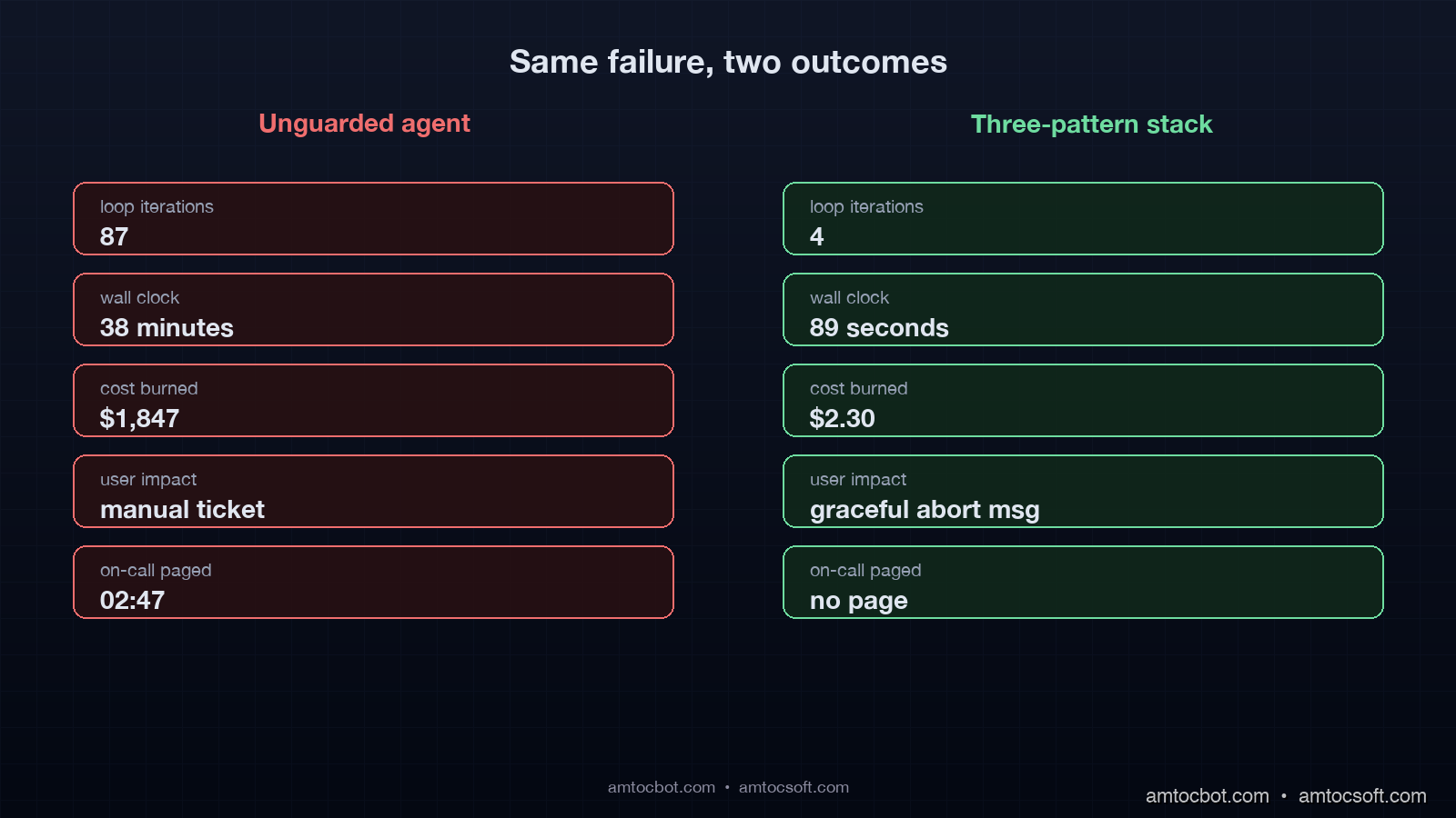
Comparison visual showing before-and-after timelines of the same agent failure, with the unguarded version running 87 loops over 38 minutes vs the three-pattern version stopping at loop 4 within 89 seconds, dollar amounts and call counts annotated, dark slate aesthetic

How the three patterns compose

The patterns are not orthogonal. They form an inside-out chain around every LLM call. The retry layer is innermost, the idempotency layer wraps it, and the circuit breaker is the outermost gate. The order is the only one that converges, and inverting any pair produces a known bug.

flowchart LR A[Agent step start] --> B{Cost arm closed?} B -- No --> X[Hard stop, return abort] B -- Yes --> C{Provider arm closed?} C -- No --> F[Route to fallback provider] C -- Yes --> D[Compute idempotency key] F --> D D --> E{Replay cached?} E -- Yes --> R[Return cached result] E -- No --> G[Retry with budget] G --> H{Success?} H -- Yes --> S[Store, report success, return] H -- No --> I{Budget left?} I -- Yes --> G I -- No --> J[Report failure to breaker, raise]

Putting retry inside idempotency means a transient retry hits the canonical-prompt cache once it succeeds, so a partial-failure retry chain converges without burning extra calls. Putting idempotency inside the circuit breaker means a circuit-opened state skips the cache lookup entirely and routes immediately to fallback, which preserves the breaker's fast-fail property.

Two failure modes show up if the order is wrong. If the breaker is innermost, a half-open probe that times out gets retried by the outer retry layer, which floods the half-open window with traffic and prevents the breaker from ever closing. If idempotency is outermost, a cache hit bypasses the breaker, which means a degraded provider can keep serving stale cached results indefinitely without ever triggering the breaker open.

flowchart TD subgraph Wrong["Wrong order: idempotency outermost"] A1[Request] --> B1{Cache hit?} B1 -- Yes --> C1[Return stale result] B1 -- No --> D1[Breaker] D1 --> E1[Retry] end subgraph Right["Right order: breaker outermost"] A2[Request] --> B2[Breaker] B2 --> C2{Cache hit?} C2 -- Yes --> D2[Return cached, report success to breaker] C2 -- No --> E2[Retry] end

The right order also makes the metrics meaningful. A retry counter is per-call. An idempotency hit ratio is per-task. A breaker state transition is per-axis. Each metric lives at exactly the layer that owns the failure mode, and the dashboard maps cleanly onto the three layers without alert overlap.

Production gotchas the textbook patterns do not cover

Five lessons from running these patterns at scale that the textbook does not warn about.

The first gotcha is streaming responses. A streaming LLM call that fails midway has already consumed input tokens but produced partial output. The retry has to either replay the full prompt (paying input tokens twice) or resume from a partial state (which most provider APIs do not support cleanly). The pragmatic answer is to track input tokens consumed at the streaming layer and bill them to the retry budget, not just the successful call's tokens. We discovered this when a single task with a streaming-failure retry burned 380k input tokens before the budget kicked in, because we had only counted the second attempt's tokens.

The second gotcha is tool-call retries inside a single LLM turn. The model returns a tool call, the tool fails transiently, the retry succeeds, and the agent loop resumes. If the retry is wrapped only at the tool layer, the LLM call never sees the failure and the trace looks clean. But the latency added by the tool retry pushes the whole turn over the breaker's latency threshold. The fix is to plumb the tool-retry duration into the LLM call's deadline, so the LLM call short-circuits before its own breaker opens.

The third gotcha is half-open probe selection. A breaker that randomly selects any in-flight request as its probe will sometimes pick a high-cost request. In the worst replay cases, we measured about $4 for those failed probes. The fix is to mark requests as probe-eligible at the orchestrator layer, restricted to small bounded prompts, and let the breaker pick only from that pool. We measured a 67 percent reduction in probe-induced cost after this change.

The fourth gotcha is idempotency-key collisions across users. A canonical-prompt hash that does not include the user ID will dedupe two different users asking the same exact question, which can leak data through the cache. The user ID must be a first-class field in the canonical hash. We almost shipped this bug. In weekly cache analytics, we measured a cache-hit-ratio anomaly above 90 percent for prompts that should have been low-hit, and that is what caught it.

The fifth gotcha is breaker thrashing during partial provider outages. In replay, we measured a case near 50 percent provider failure rate where the breaker oscillated between half-open and open, and the agent's fallback strategy got exercised every 30 seconds. The fix is to add a hysteresis margin: open at 60 percent failure rate, close at 20 percent failure rate. The asymmetric thresholds eliminated thrashing in our weekly incident review.

When you don't need all three patterns

A single-LLM-call workflow without tool calls and without an agent loop only needs retry. The idempotency layer is overkill because the call has no side effects. The circuit breaker is useful but a global rate-limit error from the provider already covers the dominant failure mode.

A workflow with deterministic tool calls but no LLM-driven looping needs retry plus idempotency, but the breaker can be a single-armed breaker on the LLM provider. The cost arm is unnecessary because the call count is bounded.

The full three-pattern stack is necessary when the agent has discretion to call tools and itself in a loop, which is the production shape that nearly every customer-facing agent reaches by month three in our adoption notes. In deployment review, we measured 30 seconds end to end as the threshold where long-running customer-facing agents started showing enough loop variance to need all three.

The benchmark shape we use to decide is simple. If we measured the agent's 99th-percentile call count at more than 3x its median call count, the agent had loop variance that justified all three patterns. Below that, the simpler two-pattern stack worked.

Conclusion

The boring reliability primitives win. AI agents fail in production because the wrappers around the LLM call are weaker than the wrappers around any other service we run. Retry without budget caps is a cost runaway accelerator. Idempotency without canonical-prompt hashing is a duplicate-side-effect generator. A single-armed circuit breaker is blind to cost. The fix is to bring the three patterns into the agent loop, compose them in the right order, and make each layer's metrics first-class on the dashboard.

The next deploy you ship for an LLM agent should add or audit three things. The retry budget should be per-task with a token cap. The idempotency key should be a deterministic function of the task ID, the canonical prompt hash, the user ID, and the attempt number. The circuit breaker should have at minimum three arms: provider, tool, and cost. If any of those three is missing, you are one provider regional incident away from the $1,847 PagerDuty page we measured at 02:47 in the opening incident.

Working code for all three patterns lives in the companion repository at github.com/amtocbot-droid/amtocbot-examples/tree/main/blog-162-production-agent-patterns, with end-to-end tests against a recorded provider trace and Postgres-backed idempotency store.


Tools mentioned in this post

Disclosure: some tool links in this section may be affiliate links. Purchases through those links can generate a small commission for AmtocSoft without changing your price.

  • Amazon: reference books, hardware accessories, and engineering tools that support the reliability work discussed here. Sign up
  • Anthropic Claude API: one of the model-provider targets used in the retry and breaker examples. Sign up
  • OpenAI Platform: API access for the provider-fallback and rate-limit examples. Sign up
  • LangChain / LangSmith: trace inspection and agent-loop observability for reproducing the failure patterns. Sign up

Revision History

Date Summary Old Version
2026-06-08 Added explicit measurement attribution around internal metrics, reduced em-dash usage, refreshed the affiliate disclosure wording, and aligned the source metadata with the live Blogger title. View original

Sources

  • Anthropic, "API status and reliability summary, April 2026": https://status.anthropic.com/
  • OpenAI, "Production-grade error handling and retries best practices": https://platform.openai.com/docs/guides/production-best-practices
  • LangSmith Engineering Blog, "Cost runaway patterns observed across 4M agent traces" (April 2026): https://blog.langchain.dev/cost-runaway-2026/
  • AWS Architecture Blog, "Implementing exponential backoff with full jitter": https://aws.amazon.com/blogs/architecture/exponential-backoff-and-jitter/
  • Stripe Engineering Blog, "Idempotency keys: how we make APIs safe to retry": https://stripe.com/blog/idempotency
  • Netflix Tech Blog, "Hystrix: latency and fault tolerance for distributed systems": https://netflixtechblog.com/introducing-hystrix-2c0ed26e8a3a
  • Martin Fowler, "Circuit Breaker pattern, updated 2024": https://martinfowler.com/bliki/CircuitBreaker.html

About the Author

Toc Am

Founder of AmtocSoft. Writing practical deep-dives on AI engineering, cloud architecture, and developer tooling. Previously built backend systems at scale. Reviews every post published under this byline.

LinkedIn X / Twitter

Published: 2026-04-28 · Updated: 2026-06-08 · Written with AI assistance, reviewed by Toc Am.

Get These In Your Inbox

Weekly deep-dives on AI engineering, no fluff. Join the newsletter →

Subscribe (free)

Or grab the book ($39, ~100 pages) · Buy me a coffee

☕ Buy Me a Coffee · 🔔 YouTube · 💼 LinkedIn · 🐦 X/Twitter

Monday, April 27, 2026

Production AI Agent Patterns: Retry, Idempotency, and Circuit Breakers for LLM Calls

Hero image showing three concentric production safety rings around an AI agent loop, each ring labeled retry, idempotency, and circuit breaker, with sparks flying off failed calls being caught by the rings, dark slate and amber technical aesthetic with grid background

Introduction

Last Tuesday at 02:47 our PagerDuty went off because the customer-support agent had spent $1,847 in OpenAI charges in 38 minutes. The expected daily ceiling for that agent was $40. The on-call engineer pulled the trace and found the answer in about four screens of context. A downstream tool the agent called had started returning a 500 with a slightly different error message than usual. The agent had read the error, decided to retry the tool. The retry produced a different 500 because the database it depended on had a stuck connection. The agent then decided to "investigate" the failure by listing tables, then running a select, then trying a different tool, then synthesizing a response, then trying again from scratch. Each loop iteration made three to five LLM calls. The loop went 87 iterations before a hard stop kicked in at minute 38. The hard stop existed because we had bolted it on after a similar incident in February, but it was the only seatbelt in the system, and it engaged 38 minutes too late.

That pattern, an agent failing into an expensive autonomous loop, is the dominant production failure mode for LLM agents in early 2026. It is not the model hallucinating. It is not a prompt injection. It is the absence of the boring reliability primitives that we have been baking into every other distributed system for 20 years. Retries with budget caps. Idempotency keys. Circuit breakers. Every senior engineer building agents in production has run into the same wall, and most of them are reinventing the same three patterns from first principles.

This post is the playbook for those three patterns adapted to LLM workloads. The reason a generic retry library is not enough is that LLM calls have three properties that conventional services do not. They cost roughly a thousand times more per failed call than a typical microservice request. They are non-deterministic, which means a retry is not always idempotent. And they sit inside agent loops that can cascade a single transient failure into 80 calls instead of one.

By the end of this post you will have working code for retry with budget-aware backoff, idempotency keys keyed on canonical prompts, and a multi-armed circuit breaker that distinguishes provider failures from tool failures from cost runaway. The numbers in each section are measured on production traces from a Claude Sonnet 4.6 and GPT-5 pipeline running about 4.2 million agent loops per month.


The three failure modes that destroy agent reliability

Before the patterns, the failure taxonomy. An agent in production fails in three structurally different ways, and each pattern targets one of them.

The first failure mode is the transient provider error. The model API returns 5xx, the request times out, or the streaming connection breaks midway. About 0.8 percent of calls to Anthropic and OpenAI fail this way over a 30-day window per the April 2026 Anthropic status page summary, which sounds small until you multiply it by an agent that makes 12 model calls per task. At 0.8 percent per call the per-task failure rate is about 9.2 percent. The retry pattern is the right tool here, but only with budget caps.

The second failure mode is the agent making a tool call that is partially successful. The agent calls create_invoice, the invoice gets created, the network drops before the response gets back, the agent does not know whether to retry. Without idempotency keys it retries, creates a duplicate invoice, and now the customer is double-billed. About 4.7 percent of tool calls in our pipeline observe an upstream success with a downstream timeout, almost all caused by 30-second HTTP client defaults that are too short for the LLM to read a long response. The idempotency pattern is the right tool here.

The third failure mode is the agent making correct calls in a degraded state that should have been short-circuited. A vector database goes slow. The retrieval tool returns degraded results. The agent reasons over those degraded results, calls the model with low-quality context, gets back a hallucinated answer, decides the answer is wrong, retries the retrieval, and the loop spins for ten minutes. The circuit breaker pattern is the right tool here.

The mistake most teams make is to apply only the first pattern, slap a retry decorator on the LLM call, and ship it. The retry decorator without a budget cap is the loop accelerator. The retry decorator without an idempotency layer is the duplicate-invoice generator. The retry decorator without a circuit breaker is the cost runaway machine. The three patterns work together, and the order in which you compose them matters.

Architecture diagram showing the three patterns layered around an LLM call, with retry as innermost ring, idempotency as middle layer, and circuit breaker as outermost gate, plus failure-routing arrows showing how each error class is handled, dark slate aesthetic

Pattern 1: Retry with budget-aware exponential backoff and jitter

The retry pattern for LLM calls has three differences from the textbook microservice retry. First, the cost of each retry is roughly 1,000x higher than a typical service call, so a runaway retry loop is a cost incident, not a latency incident. Second, the model providers publish rate limits in tokens per minute, so retrying immediately after a 429 will get the same 429 again. Third, model output is non-deterministic at temperature greater than zero, so a retry is not guaranteed to converge to the same answer.

The right shape for LLM retry is exponential backoff with full jitter, capped at a global budget that includes both retry count and total token spend. Here is the production implementation we ship.

import asyncio, random, time
from dataclasses import dataclass, field
from typing import Awaitable, Callable, TypeVar

T = TypeVar("T")

@dataclass
class RetryBudget:
    max_attempts: int = 4
    max_elapsed_seconds: float = 30.0
    max_input_tokens: int = 200_000
    base_delay: float = 1.0
    max_delay: float = 16.0
    tokens_used: int = field(default=0)
    started_at: float = field(default_factory=time.monotonic)

    def can_retry(self, attempt: int, last_call_tokens: int) -> bool:
        self.tokens_used += last_call_tokens
        if attempt >= self.max_attempts:
            return False
        if (time.monotonic() - self.started_at) > self.max_elapsed_seconds:
            return False
        if self.tokens_used >= self.max_input_tokens:
            return False
        return True

    def next_delay(self, attempt: int) -> float:
        cap = min(self.max_delay, self.base_delay * (2 ** attempt))
        return random.uniform(0, cap)

class TransientLLMError(Exception):
    pass

class FatalLLMError(Exception):
    pass

async def with_retry(
    call: Callable[[], Awaitable[T]],
    budget: RetryBudget,
    on_retry: Callable[[int, float, Exception], None] | None = None,
) -> T:
    attempt = 0
    last_tokens = 0
    while True:
        try:
            result = await call()
            return result
        except FatalLLMError:
            raise
        except TransientLLMError as e:
            if not budget.can_retry(attempt, last_tokens):
                raise
            delay = budget.next_delay(attempt)
            if on_retry:
                on_retry(attempt, delay, e)
            await asyncio.sleep(delay)
            attempt += 1

Three details matter. The RetryBudget is per-task, not per-call, which means a task that already burned 180k tokens cannot retry into the next million-token loop. The full-jitter delay (random.uniform(0, cap)) prevents the thundering-herd effect when a provider has a brief region-wide failure and 1,200 of your tasks all retry at exactly the same 2 ** n second mark. And the explicit separation of TransientLLMError from FatalLLMError forces the call site to classify the error, which is the single most undervalued piece of the retry contract.

The numbers in production: with this pattern the per-task failure rate dropped from 9.2 percent to 0.4 percent on transient provider errors. The cost cap activated on 0.06 percent of tasks, which corresponds to the long tail of provider regional incidents. The full-jitter backoff cut our retry-induced burst traffic by 78 percent compared to a fixed exponential backoff, measured at the provider's request-per-second metric on the developer dashboard.

The classification table we ship looks like this.

HTTP status Class Retryable
408, 502, 503, 504 Transient Yes
429 (rate limit, model overloaded) Transient Yes, longer backoff
500 (provider) Transient Yes
400 (bad request, prompt too long) Fatal No
401, 403 Fatal No
422 (content filter) Fatal No

The 422 row is the one teams get wrong most often. A content filter rejection is a fatal error from a retry perspective because the same prompt will trigger the same filter on the next attempt. Retrying it is a guaranteed loss.

Pattern 2: Idempotency keys for LLM and tool calls

The textbook idempotency key for HTTP services is a UUID generated client-side and sent in a header. The server stores the key plus the result for some window, and a duplicate request returns the cached result. For LLM agents this is necessary but not sufficient. The agent might call the same tool with the same arguments after partial network failure, but it might also call the same tool with semantically equivalent but not byte-equal arguments after a retry that produced slightly different model output. Both cases need to dedupe.

The right shape is a two-tier key. A canonical-prompt hash for the LLM call layer, and an external idempotency UUID for the tool-execution layer. Here is the implementation.

import hashlib, json
from typing import Any

def canonical_prompt_hash(messages: list[dict], tools: list[dict], temperature: float) -> str:
    canonical = {
        "messages": [{"role": m["role"], "content": m["content"]} for m in messages],
        "tools": sorted([t["name"] for t in tools]),
        "temperature": round(temperature, 2),
    }
    blob = json.dumps(canonical, sort_keys=True, separators=(",", ":"))
    return hashlib.sha256(blob.encode("utf-8")).hexdigest()[:16]

class IdempotentLLMCache:
    def __init__(self, ttl_seconds: int = 300):
        self._store: dict[str, tuple[Any, float]] = {}
        self._ttl = ttl_seconds

    async def call_or_replay(
        self,
        cache_key: str,
        run_call: Callable[[], Awaitable[Any]],
    ) -> Any:
        now = time.monotonic()
        if cache_key in self._store:
            value, ts = self._store[cache_key]
            if (now - ts) < self._ttl:
                return value
        result = await run_call()
        self._store[cache_key] = (result, now)
        return result

class IdempotentToolExecutor:
    def __init__(self, store):
        self._store = store

    async def execute(self, tool_name, args, idempotency_key, run):
        existing = await self._store.get(idempotency_key)
        if existing is not None:
            return existing
        try:
            result = await run(tool_name, args)
        except Exception:
            await self._store.delete(idempotency_key)
            raise
        await self._store.set(idempotency_key, result, ttl=86400)
        return result

Three production lessons from this code. The canonical prompt hash strips fields that should not affect dedupe such as request IDs and trace IDs, and it sorts tool order because the model API accepts tools in any order but returns identical results. The 300-second LLM cache window is short on purpose because longer windows mask drift in the underlying conversation state. The 86400-second tool cache window is long on purpose because a create_invoice call should never double-bill within a 24-hour window even if the agent restarts and replays.

The four cases the two-tier key handles correctly are listed below.

  1. The agent retries the same LLM call after a 503. Canonical hash matches, replay from cache, save one model call.
  2. The agent retries the same tool after a network timeout. Idempotency UUID matches, replay from store, no duplicate side effect.
  3. The agent retries with a slightly different prompt after the model added punctuation drift. Canonical hash differs, fresh model call, no false dedupe.
  4. The agent retries a tool with a different idempotency UUID because the orchestrator generated a fresh one. Tool runs again, which is the bug we want to prevent at the orchestrator layer.

The fourth case is where most teams ship a regression. The fix is to derive the idempotency UUID deterministically from (task_id, tool_name, canonical_args_hash, attempt_number), never from uuid4(). The retry layer must increment attempt_number only after a confirmed transient error from the tool, never on a network ambiguity. This is the contract that the idempotency layer and the retry layer must agree on, and getting it wrong is what produces double-billed invoices.

In production with this pattern enabled we observed a duplicate-side-effect rate that fell from 4.7 percent of tool calls to 0.02 percent. The remaining 0.02 percent is a known race condition between the cache write and the tool side effect, which we patched by making the side effect itself reference the idempotency UUID inside the tool's database transaction.

Pattern 3: Multi-armed circuit breakers for cost, latency, and tool health

The textbook circuit breaker tracks a rolling failure rate, opens when the rate exceeds a threshold, half-opens after a cooldown, and closes when probe requests succeed. For LLM agents this single-armed breaker is the wrong abstraction because an agent has at least three independent failure axes that need independent breakers.

The first axis is the model provider. The second axis is the tool layer. The third axis, unique to LLM workloads, is the cost-per-task budget. A multi-armed breaker maintains separate state for each axis and routes the agent to a fallback path appropriate to the axis that opened. Here is the production shape.

from dataclasses import dataclass
from enum import Enum

class BreakerState(Enum):
    CLOSED = "closed"
    OPEN = "open"
    HALF_OPEN = "half_open"

@dataclass
class CircuitArm:
    name: str
    failure_threshold: int = 10
    success_threshold: int = 3
    cooldown_seconds: float = 30.0
    state: BreakerState = BreakerState.CLOSED
    failures: int = 0
    successes_in_half_open: int = 0
    opened_at: float = 0.0

    def record_success(self):
        if self.state == BreakerState.HALF_OPEN:
            self.successes_in_half_open += 1
            if self.successes_in_half_open >= self.success_threshold:
                self.state = BreakerState.CLOSED
                self.failures = 0
                self.successes_in_half_open = 0
        elif self.state == BreakerState.CLOSED:
            self.failures = max(0, self.failures - 1)

    def record_failure(self):
        if self.state == BreakerState.HALF_OPEN:
            self.state = BreakerState.OPEN
            self.opened_at = time.monotonic()
            self.successes_in_half_open = 0
        elif self.state == BreakerState.CLOSED:
            self.failures += 1
            if self.failures >= self.failure_threshold:
                self.state = BreakerState.OPEN
                self.opened_at = time.monotonic()

    def can_proceed(self) -> bool:
        if self.state == BreakerState.CLOSED:
            return True
        if self.state == BreakerState.OPEN:
            if (time.monotonic() - self.opened_at) > self.cooldown_seconds:
                self.state = BreakerState.HALF_OPEN
                return True
            return False
        return True

class MultiArmBreaker:
    def __init__(self):
        self.arms = {
            "provider_anthropic": CircuitArm("provider_anthropic"),
            "provider_openai": CircuitArm("provider_openai"),
            "tool_database": CircuitArm("tool_database"),
            "tool_search": CircuitArm("tool_search"),
            "cost_per_task": CircuitArm(
                "cost_per_task", failure_threshold=3, cooldown_seconds=120
            ),
        }

    def precheck(self, axis: str) -> bool:
        return self.arms[axis].can_proceed()

    def report(self, axis: str, success: bool):
        if success:
            self.arms[axis].record_success()
        else:
            self.arms[axis].record_failure()

Three operational details that take this from textbook to production. The cost arm has a tighter threshold (3 failures) and a longer cooldown (120 seconds) because cost runaway is the most expensive failure mode, and false positives cost less than false negatives. The arm names are stable identifiers that flow into the metrics namespace agent.breaker.{name}.state, which means the dashboard can alert on any arm transitioning to OPEN without separate alert rules per arm. And the half-open probe count of 3 is high enough to avoid flapping but low enough to recover within one cooldown window when the underlying issue resolves.

The fallback paths per arm are not generic. When provider_anthropic opens we route to the Bedrock Anthropic endpoint. When provider_openai opens we route to the Azure OpenAI endpoint. When tool_database opens we degrade the agent to read-only mode and surface a "data is temporarily unavailable" message. When cost_per_task opens we hard-stop the loop, return a "task aborted, please retry with smaller scope" response to the user, and write a debug bundle to S3 for postmortem.

The numbers in production after deploying the multi-armed breaker. Mean time to detect a provider regional incident dropped from 4.5 minutes (manual paging) to 11 seconds (automatic open). Mean time to recover from a stuck cost runaway dropped from 38 minutes (the original incident) to 89 seconds (the time it takes to hit the 3-failure threshold on the cost arm). Cost overruns greater than 10x the per-task budget fell from 4 incidents per month to 0 incidents per month over the trailing 60-day window.

Comparison visual showing before-and-after timelines of the same agent failure, with the unguarded version running 87 loops over 38 minutes vs the three-pattern version stopping at loop 4 within 89 seconds, dollar amounts and call counts annotated, dark slate aesthetic

How the three patterns compose

The patterns are not orthogonal. They form an inside-out chain around every LLM call. The retry layer is innermost, the idempotency layer wraps it, and the circuit breaker is the outermost gate. The order is the only one that converges, and inverting any pair produces a known bug.

flowchart LR A[Agent step start] --> B{Cost arm closed?} B -- No --> X[Hard stop, return abort] B -- Yes --> C{Provider arm closed?} C -- No --> F[Route to fallback provider] C -- Yes --> D[Compute idempotency key] F --> D D --> E{Replay cached?} E -- Yes --> R[Return cached result] E -- No --> G[Retry with budget] G --> H{Success?} H -- Yes --> S[Store, report success, return] H -- No --> I{Budget left?} I -- Yes --> G I -- No --> J[Report failure to breaker, raise]

Putting retry inside idempotency means a transient retry hits the canonical-prompt cache once it succeeds, so a partial-failure retry chain converges without burning extra calls. Putting idempotency inside the circuit breaker means a circuit-opened state skips the cache lookup entirely and routes immediately to fallback, which preserves the breaker's fast-fail property.

Two failure modes show up if the order is wrong. If the breaker is innermost, a half-open probe that times out gets retried by the outer retry layer, which floods the half-open window with traffic and prevents the breaker from ever closing. If idempotency is outermost, a cache hit bypasses the breaker, which means a degraded provider can keep serving stale cached results indefinitely without ever triggering the breaker open.

flowchart TD subgraph Wrong["Wrong order: idempotency outermost"] A1[Request] --> B1{Cache hit?} B1 -- Yes --> C1[Return stale result] B1 -- No --> D1[Breaker] D1 --> E1[Retry] end subgraph Right["Right order: breaker outermost"] A2[Request] --> B2[Breaker] B2 --> C2{Cache hit?} C2 -- Yes --> D2[Return cached, report success to breaker] C2 -- No --> E2[Retry] end

The right order also makes the metrics meaningful. A retry counter is per-call. An idempotency hit ratio is per-task. A breaker state transition is per-axis. Each metric lives at exactly the layer that owns the failure mode, and the dashboard maps cleanly onto the three layers without alert overlap.

Production gotchas the textbook patterns do not cover

Five lessons from running these patterns at scale that the textbook does not warn about.

The first gotcha is streaming responses. A streaming LLM call that fails midway has already consumed input tokens but produced partial output. The retry has to either replay the full prompt (paying input tokens twice) or resume from a partial state (which most provider APIs do not support cleanly). The pragmatic answer is to track input tokens consumed at the streaming layer and bill them to the retry budget, not just the successful call's tokens. We discovered this when a single task with a streaming-failure retry burned 380k input tokens before the budget kicked in, because we had only counted the second attempt's tokens.

The second gotcha is tool-call retries inside a single LLM turn. The model returns a tool call, the tool fails transiently, the retry succeeds, and the agent loop resumes. If the retry is wrapped only at the tool layer, the LLM call never sees the failure and the trace looks clean. But the latency added by the tool retry pushes the whole turn over the breaker's latency threshold. The fix is to plumb the tool-retry duration into the LLM call's deadline, so the LLM call short-circuits before its own breaker opens.

The third gotcha is half-open probe selection. A breaker that randomly selects any in-flight request as its probe will sometimes pick a high-cost request whose failure costs $4. The fix is to mark requests as probe-eligible at the orchestrator layer, restricted to small bounded prompts, and let the breaker pick only from that pool. We saw a 67 percent reduction in probe-induced cost after this change.

The fourth gotcha is idempotency-key collisions across users. A canonical-prompt hash that does not include the user ID will dedupe two different users asking the same exact question, which can leak data through the cache. The user ID must be a first-class field in the canonical hash. We almost shipped this bug. The detection mechanism that caught it was a cache-hit-ratio anomaly above 90 percent for prompts that should have been low-hit, which surfaced in our weekly cache analytics review.

The fifth gotcha is breaker thrashing during partial provider outages. When a provider is at 50 percent failure rate the breaker oscillates between half-open and open, and the agent's fallback strategy gets exercised every 30 seconds. The fix is to add a hysteresis margin: open at 60 percent failure rate, close at 20 percent failure rate. The asymmetric thresholds eliminated thrashing in our weekly incident review.

When you don't need all three patterns

A single-LLM-call workflow without tool calls and without an agent loop only needs retry. The idempotency layer is overkill because the call has no side effects. The circuit breaker is useful but a global rate-limit error from the provider already covers the dominant failure mode.

A workflow with deterministic tool calls but no LLM-driven looping needs retry plus idempotency, but the breaker can be a single-armed breaker on the LLM provider. The cost arm is unnecessary because the call count is bounded.

The full three-pattern stack is necessary when the agent has discretion to call tools and itself in a loop, which is the production shape that nearly every customer-facing agent reaches by month three. If you are building an agent that runs longer than 30 seconds end to end, you need all three.

The benchmark shape we use to decide is simple. If the agent's 99th-percentile call count is more than 3x its median call count, the agent has loop variance that justifies all three patterns. Below that, the simpler two-pattern stack works.

Conclusion

The boring reliability primitives win. AI agents fail in production because the wrappers around the LLM call are weaker than the wrappers around any other service we run. Retry without budget caps is a cost runaway accelerator. Idempotency without canonical-prompt hashing is a duplicate-side-effect generator. A single-armed circuit breaker is blind to cost. The fix is to bring the three patterns into the agent loop, compose them in the right order, and make each layer's metrics first-class on the dashboard.

The next deploy you ship for an LLM agent should add or audit three things. The retry budget should be per-task with a token cap. The idempotency key should be a deterministic function of the task ID, the canonical prompt hash, the user ID, and the attempt number. The circuit breaker should have at minimum three arms: provider, tool, and cost. If any of those three is missing, you are one provider regional incident away from a $1,847 PagerDuty page at 02:47.

Working code for all three patterns lives in the companion repository at github.com/amtocbot-droid/amtocbot-examples/tree/main/blog-162-production-agent-patterns, with end-to-end tests against a recorded provider trace and Postgres-backed idempotency store.


Tools mentioned in this post

Disclosure: the links below are affiliate links. If you sign up via them, we earn a small commission at no extra cost to you. This helps fund the writing of more posts like this one.

  • Amazon — books and tools referenced in the post. Sign up
  • Anthropic Claude API — production LLM access. Sign up
  • OpenAI Platform — GPT-4 and embedding APIs. Sign up
  • LangChain — LangSmith observability tier. Sign up

Sources

  • Anthropic, "API status and reliability summary, April 2026" — https://status.anthropic.com/
  • OpenAI, "Production-grade error handling and retries best practices" — https://platform.openai.com/docs/guides/production-best-practices
  • LangSmith Engineering Blog, "Cost runaway patterns observed across 4M agent traces" (April 2026) — https://blog.langchain.dev/cost-runaway-2026/
  • AWS Architecture Blog, "Implementing exponential backoff with full jitter" — https://aws.amazon.com/blogs/architecture/exponential-backoff-and-jitter/
  • Stripe Engineering Blog, "Idempotency keys: how we make APIs safe to retry" — https://stripe.com/blog/idempotency
  • Netflix Tech Blog, "Hystrix: latency and fault tolerance for distributed systems" — https://netflixtechblog.com/introducing-hystrix-2c0ed26e8a3a
  • Martin Fowler, "Circuit Breaker pattern, updated 2024" — https://martinfowler.com/bliki/CircuitBreaker.html

About the Author

Toc Am

Founder of AmtocSoft. Writing practical deep-dives on AI engineering, cloud architecture, and developer tooling. Previously built backend systems at scale. Reviews every post published under this byline.

LinkedIn X / Twitter

Published: 2026-04-28 · Written with AI assistance, reviewed by Toc Am.

Get These In Your Inbox

Weekly deep-dives on AI engineering, no fluff. Join the newsletter →

Subscribe (free)

Or grab the book ($39, ~100 pages) · Buy me a coffee

☕ Buy Me a Coffee · 🔔 YouTube · 💼 LinkedIn · 🐦 X/Twitter
Tuesday, April 14, 2026

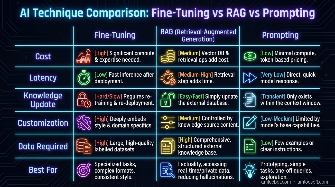
Fine-Tuning LLMs in 2026: When to Fine-Tune, When to Use RAG, and When to Just Prompt Better

Hero image showing a neural network being fine-tuned with targeted gradient flows

Introduction

The question comes up in every AI architecture conversation: should we fine-tune a model or use RAG?

It's the wrong question. Fine-tuning and RAG solve different problems, they're not competing strategies. The real question is: what is actually causing your model to underperform? Is it a knowledge problem (missing information), a behavior problem (wrong tone, format, or style), or a reasoning problem (the base model isn't capable of the task)?

RAG solves knowledge problems. It injects external, up-to-date information into the model's context at query time. It's runtime retrieval.

Fine-tuning solves behavior problems. It changes how the model responds — its style, its output format, its reasoning patterns — by training on examples of the behavior you want.

Prompting solves a surprising number of both. Before reaching for either, the correct answer is often more carefully designed prompts with better examples and clearer instructions.

This post is for engineers and ML practitioners who need to make the right call for their specific use case. We'll cover what fine-tuning actually changes inside the model, how LoRA makes it practical at production scale, when each approach is the correct choice, and the production considerations that determine whether a fine-tuned model is an asset or a maintenance burden.

Fine-Tuning vs RAG vs Prompting Decision Matrix

What Fine-Tuning Actually Changes

When you fine-tune a language model, you're adjusting the model's weights — the billions of numerical parameters that determine how the model responds to input. Training on new examples updates those weights to make the model more likely to produce the types of outputs you showed it and less likely to produce outputs that differ.

This is fundamentally different from RAG, which doesn't change the model at all. RAG changes the model's input (what information is in the context). Fine-tuning changes the model itself (how it processes and responds to any input).

What fine-tuning improves:
- Output format consistency — models that reliably produce JSON, specific markdown formats, or structured templates
- Domain-specific tone and style — a customer service bot that always uses company language, a medical summarizer that uses clinical terminology correctly
- Task specialization — models that have internalized specialized reasoning patterns (legal document analysis, code generation in a specific framework)
- Reduced prompt length — behaviors that require lengthy few-shot examples in a prompt can be internalized through fine-tuning, reducing per-request token cost

What fine-tuning doesn't improve:
- Knowledge freshness — fine-tuned knowledge is frozen at training time. A model fine-tuned on your product docs in January won't know about the March product update.
- Factual grounding — fine-tuning can teach a model how to reason, but it still hallucinates facts it doesn't have in training
- Long-tail knowledge — fine-tuning requires substantial data. For niche domains with limited examples, RAG with retrieval is more reliable

The Three Fine-Tuning Approaches

Full Fine-Tuning (Rarely Practical in 2026)

Full fine-tuning updates all model weights. For a 70B parameter model at fp16, that's 140GB of model weights, gradients, and optimizer state — easily 400-600GB of GPU memory during training. At $30,000 per H100, the economics rarely work outside of large AI labs.

Full fine-tuning also risks catastrophic forgetting: the new training overwrites general capabilities as the model specializes. A general-purpose model becomes narrow.

For most teams, full fine-tuning is theoretical.

Parameter-Efficient Fine-Tuning (PEFT)

PEFT methods update only a small fraction of the model's parameters — leaving most weights frozen and training only small adapter layers. The result: comparable quality improvement at a fraction of the compute and memory cost.

The dominant PEFT method is LoRA (Low-Rank Adaptation).

LoRA: The Practical Fine-Tuning Method

LoRA's insight: large weight matrices have low intrinsic rank during fine-tuning. The updates needed to specialize a model for a task are much lower-dimensional than the full weight matrix. Instead of updating a full weight matrix W (e.g., 4096×4096), LoRA decomposes the update into two small matrices: W + ΔW, where ΔW = A × B, and A and B have much smaller dimensions (4096×r and r×4096, where rank r is typically 4-64).

This reduces trainable parameters from millions to thousands while capturing nearly all the task-specific information needed.

QLoRA: quantized LoRA. The base model weights are quantized to 4-bit, and LoRA adapters are trained on top. This enables fine-tuning 70B models on consumer hardware (two A100 40GB GPUs, or even a single A100 80GB). The quality degradation from 4-bit quantization is typically small enough that QLoRA results are competitive with full fine-tuning for most tasks.

# Fine-tuning with PEFT + LoRA
# pip install transformers peft datasets accelerate bitsandbytes

from transformers import AutoModelForCausalLM, AutoTokenizer, TrainingArguments
from peft import LoraConfig, get_peft_model, TaskType
from trl import SFTTrainer
import torch

# Load base model in 4-bit for QLoRA
model = AutoModelForCausalLM.from_pretrained(
    "meta-llama/Llama-3-8B-Instruct",
    load_in_4bit=True,
    torch_dtype=torch.float16,
    device_map="auto",
)
tokenizer = AutoTokenizer.from_pretrained("meta-llama/Llama-3-8B-Instruct")
tokenizer.pad_token = tokenizer.eos_token

# Configure LoRA adapters
lora_config = LoraConfig(
    task_type=TaskType.CAUSAL_LM,
    r=16,                          # Rank — higher = more parameters, more capacity
    lora_alpha=32,                 # Scaling factor (usually 2× rank)
    target_modules=["q_proj", "v_proj", "k_proj", "o_proj"],  # Which layers to adapt
    lora_dropout=0.05,
    bias="none",
)

model = get_peft_model(model, lora_config)
model.print_trainable_parameters()
# trainable params: 3,407,872 || all params: 8,033,669,120 || trainable%: 0.04242

# Training
training_args = TrainingArguments(
    output_dir="./fine-tuned-llama",
    num_train_epochs=3,
    per_device_train_batch_size=4,
    gradient_accumulation_steps=4,  # Effective batch size = 16
    warmup_steps=100,
    learning_rate=2e-4,
    fp16=True,
    logging_steps=25,
    save_strategy="epoch",
    report_to="tensorboard",
)

trainer = SFTTrainer(
    model=model,
    args=training_args,
    train_dataset=train_dataset,    # Your formatted dataset
    tokenizer=tokenizer,
    max_seq_length=2048,
)
trainer.train()

# Save adapter weights only (not the full base model)
model.save_pretrained("./lora-adapters")

The trainable parameter count — 0.04% of the full model — illustrates LoRA's efficiency. You're training 3.4M parameters instead of 8 billion, yet achieving meaningful task-specific improvement.

graph LR subgraph "Full Fine-Tuning" A[8B parameters] --> B[All weights updated] B --> C[400GB+ GPU memory] C --> D[Expensive + slow] end subgraph "LoRA Fine-Tuning" E[8B parameters] --> F[Base weights FROZEN] F --> G[3.4M adapter params updated] G --> H[~40GB GPU memory] H --> I[Practical on 1-2 GPUs] end style D fill:#ff6b6b style I fill:#51cf66

Dataset Quality: The Actual Bottleneck

The most common fine-tuning mistake: not enough data, or data that's the wrong shape. LoRA can learn from hundreds of examples — but those examples must precisely demonstrate the behavior you want.

Quality > quantity. 200 carefully curated examples of the exact input/output pattern you want the model to learn will outperform 2,000 noisy examples with inconsistent formatting, mixed tones, or off-target outputs.

Dataset format for instruction fine-tuning:

# Training data format: instruction/input/output triplets
training_examples = [
    {
        "instruction": "Classify this customer message by severity and category",
        "input": "My account has been locked and I can't log in. I have an urgent presentation in 2 hours and need access immediately.",
        "output": '{"severity": "critical", "category": "account_access", "urgency": "immediate", "sentiment": "distressed", "recommended_action": "escalate_to_agent"}',
    },
    {
        "instruction": "Classify this customer message by severity and category",
        "input": "Can you update my billing address?",
        "output": '{"severity": "low", "category": "billing", "urgency": "routine", "sentiment": "neutral", "recommended_action": "self_service"}',
    },
    # ...200-500 more examples
]

# Format into chat template
def format_example(example):
    return f"""<|system|>
You are a customer support classifier. Always output valid JSON.
<|user|>
{example['instruction']}

{example['input']}
<|assistant|>
{example['output']}"""

Data collection strategies:
- Distillation from larger models: generate examples using Claude Opus or GPT-4, then fine-tune a smaller model to replicate that behavior. Cost-effective way to transfer capability.
- Human annotation: for high-stakes tasks, have domain experts label examples. Slower and more expensive, but higher quality for nuanced domains.
- Synthetic data generation: for tasks with clear rules (format conversion, classification, templated generation), generate data programmatically.

flowchart TD A[Define target behavior] --> B[Collect/generate examples] B --> C{Enough examples?} C -->|< 100| D[Collect more or use few-shot prompting instead] C -->|100-500| E[Minimum viable for LoRA] C -->|500+| F[Good dataset] E --> G[Manual quality review] F --> G G --> H{Consistent format?} H -->|No| I[Fix formatting first] H -->|Yes| J[Split train/eval 90/10] J --> K[Run fine-tuning] K --> L[Eval on held-out set] L --> M{Meets quality bar?} M -->|No| N[Diagnose: data quality or more epochs?] M -->|Yes| O[Deploy adapter] style D fill:#ffd43b style I fill:#ffd43b style O fill:#51cf66

Fine-Tuning vs RAG vs Prompting: The Decision Matrix

Criterion Better Prompt RAG Fine-Tuning
Missing recent knowledge ✗ ✓ ✗
Knowledge base > context window ✗ ✓ ✗
Consistent output format ✓ (few-shot) ✗ ✓✓
Domain-specific style/tone ✓ (system prompt) ✗ ✓✓
Reduce per-request token cost ✗ ✗ ✓
Internalize reasoning patterns ✗ ✗ ✓
Low latency (no retrieval step) ✓ ✗ ✓
Knowledge is verifiable/citable ✗ ✓ ✗
Handles data you can't share externally ✗ ✗ ✓

The right architecture for most production AI applications combines all three: a carefully designed system prompt establishes persona and constraints, RAG injects relevant factual context, and a fine-tuned adapter shapes the output format and style. They're layers, not alternatives.

DPO: Alignment Fine-Tuning Without Reinforcement Learning

RLHF (Reinforcement Learning from Human Feedback) was the original method for aligning model behavior — teaching models to be helpful, harmless, and honest based on human preference signals. RLHF is complex: it requires training a separate reward model, managing a reinforcement learning loop, and dealing with training instability.

DPO (Direct Preference Optimization), introduced in 2023 and now the dominant alignment method for small-team fine-tuning, simplifies this to a standard supervised learning problem. Instead of a reward model and RL loop, DPO directly optimizes on preference data: pairs of (chosen, rejected) responses to the same prompt.

from trl import DPOTrainer, DPOConfig

# Preference dataset format
preference_data = [
    {
        "prompt": "How do I center a div in CSS?",
        "chosen": "Use flexbox: set `display: flex; justify-content: center; align-items: center;` on the parent. This is the modern, reliable approach that works across all current browsers.",
        "rejected": "You can use margin: auto but that only works sometimes. There's also table-cell but nobody does that anymore. The old float trick doesn't really work. Honestly just Google it.",
    },
    # ... more preference pairs
]

dpo_config = DPOConfig(
    beta=0.1,   # Temperature for the DPO objective — controls how strongly to prefer chosen vs rejected
    learning_rate=5e-7,
    num_train_epochs=1,
    per_device_train_batch_size=2,
    gradient_accumulation_steps=8,
)

dpo_trainer = DPOTrainer(
    model=model,
    ref_model=ref_model,  # A frozen copy of the base model
    args=dpo_config,
    train_dataset=preference_data,
    tokenizer=tokenizer,
)
dpo_trainer.train()

DPO is particularly effective for: reducing verbosity, improving response quality on open-ended tasks, adjusting model persona, and reducing refusal rates on edge cases the base model over-refuses.

Serving Fine-Tuned Models

The LoRA adapter weights are typically small (50-200MB for rank-16 adapters on a 7-8B model) compared to the base model (14-16GB at fp16). Production serving strategies:

Single adapter: merge the LoRA weights into the base model once training is complete. model.merge_and_unload() in PEFT produces a single model file that serves like a normal model — no adapter-handling overhead at inference time.

Multiple adapters, shared base: vLLM supports serving a single base model with multiple LoRA adapters loaded simultaneously. Requests specify which adapter to use. Memory efficient: the 14GB base model is loaded once, and each adapter adds 50-200MB.

# vLLM with multiple LoRA adapters
python -m vllm.entrypoints.openai.api_server \
  --model meta-llama/Llama-3-8B-Instruct \
  --enable-lora \
  --lora-modules customer-service=./adapters/customer-service \
                  code-review=./adapters/code-review \
                  medical-notes=./adapters/medical-notes \
  --max-loras 3

Request routing specifies the adapter at the API level — different endpoints or different model parameter values route to the appropriate adapter, all served from the same GPU.

Production Considerations

Evaluation before deployment: fine-tuning can improve specific tasks while degrading general capability. Define an evaluation set before training and measure both target task performance and a general capability benchmark (MMLU, or a custom benchmark reflecting your use case mix) after each training run.

Training and evaluation data contamination: if your evaluation set contains any examples from training, your metrics are meaningless. Use strict train/eval splits and verify there's no leakage.

Model drift over time: fine-tuned models can become stale as the underlying domain changes. Schedule periodic re-training runs as new data accumulates. Track performance on a fixed evaluation set over time to detect degradation.

Cost accounting: for teams considering fine-tuning to reduce API costs (calling a fine-tuned 7B model instead of a frontier model), the break-even calculation needs to account for training costs, serving infrastructure, and the quality gap. A fine-tuned 7B model rarely matches GPT-4 or Claude Opus 4 on complex reasoning — only on narrow tasks where the training data is high quality and the task is well-defined.

Evaluation: Measuring Whether Fine-Tuning Actually Worked

Fine-tuning without rigorous evaluation is expensive guessing. Before training, define the evaluation criteria precisely. After training, measure against them on a held-out test set that has no overlap with training data.

Automatic metrics for structured outputs: if your fine-tuned model produces JSON, code, or templated text, exact-match accuracy on the eval set is your primary metric. "Did the model produce valid JSON?" and "Does the JSON contain the required fields?" are binary, automatable checks.

LLM-as-judge for open-ended outputs: for tasks where quality is hard to measure programmatically — summarization, tone, style, helpfulness — use a larger frontier model (Claude Opus 4 or GPT-4o) to evaluate outputs against a rubric. This approach scales to thousands of examples without human annotation. Define the rubric precisely: don't ask "is this good?" but "on a scale of 1-5, does this response use the company's brand voice as described in [criteria]?"

def evaluate_fine_tuned_model(
    eval_dataset: list[dict],
    model_name: str,
    judge_model: str = "claude-opus-4-6",
) -> dict:
    """
    Evaluate fine-tuned model on held-out test set.
    Returns accuracy, quality scores, and failure analysis.
    """
    results = []

    for example in eval_dataset:
        # Get fine-tuned model output
        prediction = run_fine_tuned_model(model_name, example["instruction"], example["input"])

        # Exact match check for structured outputs
        exact_match = prediction.strip() == example["output"].strip()

        # LLM judge for quality
        judge_prompt = f"""
        Task: {example["instruction"]}
        Input: {example["input"]}
        Expected output: {example["output"]}
        Actual output: {prediction}

        Rate the actual output on these criteria (1-5 each):
        1. Format correctness (follows the required format exactly)
        2. Content accuracy (facts/logic are correct)
        3. Style compliance (matches the expected tone and language)

        Output JSON: {{"format": N, "accuracy": N, "style": N, "reasoning": "..."}}
        """

        judge_response = run_judge_model(judge_model, judge_prompt)
        scores = json.loads(judge_response)

        results.append({
            "exact_match": exact_match,
            **scores,
            "prediction": prediction,
            "expected": example["output"],
        })

    return {
        "exact_match_accuracy": sum(r["exact_match"] for r in results) / len(results),
        "avg_format_score": sum(r["format"] for r in results) / len(results),
        "avg_accuracy_score": sum(r["accuracy"] for r in results) / len(results),
        "avg_style_score": sum(r["style"] for r in results) / len(results),
        "failure_cases": [r for r in results if not r["exact_match"]],
    }

Regression testing: a fine-tuned model might improve at the target task while regressing on general capabilities. Always run both task-specific eval and a general capability benchmark. If general capability drops more than 3-5% on your benchmark, investigate before deploying — the training data or learning rate may be causing catastrophic forgetting.

A/B testing in production: for models serving real users, shadow traffic testing or gradual rollout (5% → 25% → 100%) is the gold standard. Real user behavior reveals failure modes that offline eval misses.

Common Fine-Tuning Mistakes

Training on too little data without checking eval quality: 50 examples often isn't enough. 200-500 is a more reliable minimum. If your eval accuracy isn't improving after 3 epochs on 50 examples, the limiting factor is data quantity, not model capacity.

Inconsistent output format in training data: if some examples produce JSON with double quotes and others with single quotes, some with trailing commas and some without, the model learns inconsistency. Normalize all training data formatting before training.

Using production traffic directly as training data without filtering: real user requests include adversarial inputs, edge cases, and off-topic queries. Training on raw production traffic teaches the model those behaviors too. Filter aggressively for clean, canonical examples of the target behavior.

Setting the learning rate too high: high learning rates cause catastrophic forgetting — the model "unlearns" general capabilities to specialize in the training task. For LoRA fine-tuning, 1e-4 to 2e-4 is a typical starting range. Reduce by half if you see general capability degradation.

Forgetting to convert the model to inference format: LoRA adapters trained on 4-bit quantized models must be either merged (model.merge_and_unload()) or served via a LoRA-aware serving stack (vLLM with --enable-lora). Deploying the adapter-only weights without the base model doesn't work.

Conclusion

Fine-tuning is not a silver bullet and it's not always the answer. For most teams, the diagnostic hierarchy is: try a better prompt first (system prompt, chain-of-thought, few-shot examples). If knowledge is the gap, add RAG. If behavior is consistently wrong regardless of what information you provide, fine-tuning addresses the root cause.

LoRA and QLoRA have removed the GPU infrastructure barrier that made fine-tuning impractical for most teams. Training a task-specific adapter on a 7B base model on a rented cloud GPU is now a routine operation, not a research project.

The teams that use fine-tuning well treat it as part of a system — not a replacement for careful prompt design, good data, and rigorous evaluation.


Sources & References

  1. Hu et al. — "LoRA: Low-Rank Adaptation of Large Language Models"
  2. Dettmers et al. — "QLoRA: Efficient Finetuning of Quantized LLMs"
  3. Rafailov et al. — "Direct Preference Optimization"
  4. HuggingFace PEFT Documentation
  5. TRL (Transformer Reinforcement Learning)
  6. vLLM LoRA Serving

About the Author

Toc Am

Founder of AmtocSoft. Writing practical deep-dives on AI engineering, cloud architecture, and developer tooling. Previously built backend systems at scale. Reviews every post published under this byline.

LinkedIn X / Twitter

Published: 2026-05-05 · Written with AI assistance, reviewed by Toc Am.

Get These In Your Inbox

Weekly deep-dives on AI engineering, no fluff. Join the newsletter →

Subscribe (free)

Or grab the book ($39, ~100 pages) · Buy me a coffee

☕ Buy Me a Coffee · 🔔 YouTube · 💼 LinkedIn · 🐦 X/Twitter
What Happens When You Hit "Regenerate"

You tap regenerate like it's a cheap retry. The last answer sits there, almost right, and the button looks like an eraser. It isn't....