There is a line between using AI and building with AI. On one side, you are handing a task to a model and reading the output. On the other, you have designed a system where the model reasons, decides, calls external tools, observes the results, and keeps going until the job is done — without you in the loop for every step.
That second thing is AI agent engineering. And in 2026, it has become one of the most consequential technical disciplines in software development, attracting serious investment, producing serious failures, and demanding a new category of engineering skills that most teams are still figuring out.
This post is the map. It covers what agent engineering actually is, why it is harder than regular LLM application development, how to design the full stack from foundation model to production security, and where to go deeper on each component. If you are building agents or planning to, start here.
What Is AI Agent Engineering?
The word "agent" gets applied to everything from a simple chatbot with memory to an autonomous system running multi-week research projects. That ambiguity is a problem. For this guide, here is a working definition precise enough to be useful:
An AI agent is a system in which a language model drives an autonomous execution loop — repeatedly reasoning, selecting tools, taking actions in the real world, observing results, and deciding what to do next — until a goal is reached or a stopping condition is met.
Four components are essential:
- LLM core — the model doing the reasoning, planning, and decision-making
- Tool layer — the external capabilities the agent can invoke (APIs, file systems, code interpreters, databases, browsers, other models)
- Memory layer — what the agent knows and remembers across turns (conversation history, retrieved documents, external state)
- Execution loop — the mechanism that keeps the cycle running, manages state, and handles failures
A chatbot is not an agent under this definition. A chatbot responds. An agent acts. That distinction is not semantic — it is the entire reason agent engineering requires different skills, different architectures, and different production practices than building a chat interface over GPT-4.
The diagram above is the anatomy of a production agent. Every component in it is an engineering problem with non-trivial solutions. The rest of this guide covers each one.
If you are newer to the concept and want to build a solid conceptual foundation first, What Are AI Agents? is the right starting point.
Why Agent Engineering Is Different
Building a stateless LLM application is relatively forgiving. You send a prompt, you get a completion, you display it. If the answer is wrong, the user asks again. The worst outcome is a bad answer.
Agents change the failure calculus entirely. When a model is driving a multi-step execution loop with real-world side effects, failures compound in ways that are qualitatively different from a chat completion going sideways.
Non-Determinism at Scale
LLMs are probabilistic. A single generation may produce slightly different tool call sequences across runs even with identical inputs. In a stateless chat app, this is fine — each response is independent. In an agent loop that runs fifty steps over two hours, small non-determinism early in the sequence can cascade into wildly divergent outcomes. You cannot reliably reproduce failures, which makes debugging exceptionally hard.
Real-World Side Effects
Agents call APIs. They write files, send emails, execute database transactions, submit form data, make purchases. These are not idempotent read operations. A hallucinated tool argument that sends a malformed API request to a payment processor or deletes the wrong row in a database is not a "bad answer" — it is a real incident with real consequences. The blast radius of an agent failure scales with the permissions you have granted it.
Long-Running State Management
A well-designed agent might run for minutes. A poorly designed one might be expected to run for hours. The longer an agent runs, the more ways its state can become inconsistent with the world. Processes crash. Network timeouts occur. Context windows fill up. The LLM starts "forgetting" things it knew twenty tool calls ago. Managing state across a long-running autonomous execution is a distributed systems problem, not just a prompt engineering problem.
Failure Cascades
When tool call three in a twenty-step plan fails, what happens to tool calls four through twenty? A naive implementation crashes or silently continues with bad state. A well-engineered one has compensating logic, retry strategies, and the ability to recognize when forward progress is no longer safe. This requires explicit failure handling at the orchestration layer, not just at the LLM level.
Security Surface Explosion
Every tool you give an agent is an attack surface. Every external input the agent processes — web pages, documents, API responses, user messages — is a potential prompt injection vector. Agents with broad permissions executing actions on behalf of users create privilege escalation risks that did not exist in stateless applications. Security is not a post-launch concern for agents; it must be designed in from the start.
The Agent Stack in 2026
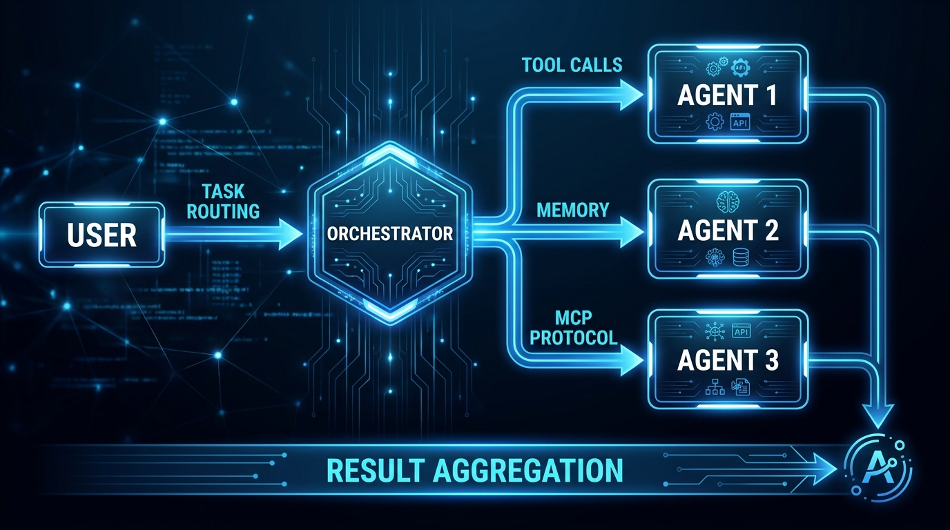
Production-grade agent systems are built in layers. Understanding each layer helps you make the right architectural choices and debug the right level when things go wrong.
Layer 1: Foundation Models
Not all LLMs are equal as agent cores. The properties that matter most for agents are distinct from properties that matter for summarization or content generation:
Tool use quality is the single most important axis. Can the model reliably produce well-formed JSON function calls? Does it understand when to use a tool versus when to answer from its own knowledge? Does it correctly chain tool calls when multiple steps are needed? As of 2026, GPT-4o, Claude 3.7 Sonnet, and Gemini 2.5 Pro are the leaders here. Smaller models are catching up but still fail on complex multi-tool orchestration.
Context length determines how much history, retrieved information, and intermediate state the model can hold. For simple two- or three-step agents, 32K tokens is sufficient. For long-running agents with large memory contexts, 128K to 200K becomes necessary. The raw number matters less than the model's ability to actually attend to information late in a long context (the "lost in the middle" problem affects some models significantly).
Instruction following — specifically the ability to adhere to structured output formats, respect system-level constraints, and maintain role fidelity across a long session — separates reliable agent cores from ones that drift off-task.
Latency and cost per call compound across an agent run. An agent that makes thirty LLM calls at $0.015 per call costs very differently than one using a smaller, faster model for intermediate steps. Routing simple reasoning steps to a smaller model and reserving the flagship model for high-stakes decisions is a pattern worth building into your architecture early.
Layer 2: Orchestration Frameworks
The orchestration layer is where your agent's logic lives — the planning, routing, memory management, and execution coordination code that sits between the LLM and everything else.
| Framework | Model | Best For | Maturity | Production Readiness |
|---|---|---|---|---|
| LangGraph | Graph-based state machine | Complex multi-step agents with explicit state, branching, and cycles | High | Strong — widely deployed in production |
| AutoGen | Multi-agent conversation | Multi-agent systems where agents communicate as peers | High | Good — Microsoft-backed, active community |
| CrewAI | Role-based agent crews | Structured multi-agent pipelines with defined roles | Medium | Growing — simpler to start, less flexible |
| OpenAI Agents SDK | Handoff-based routing | OpenAI ecosystem, simple handoff patterns | Medium | Good for GPT-4o-centric stacks |
| Bare Python | Custom | Maximum control, specialized systems | N/A | As production-ready as you make it |
LangGraph is the right choice when you need explicit control over state transitions — when your agent has well-defined phases, needs to loop back to earlier states based on observations, or needs to run parallel sub-graphs. The graph abstraction makes complex flows auditable and testable.
AutoGen works well when you want multiple specialized agents collaborating — a researcher, a coder, a critic — and you want them to communicate in natural language rather than through a rigid handoff protocol. It mirrors how human teams divide work.
CrewAI is the fastest path from zero to a working multi-agent crew for teams that value simplicity over flexibility. It handles common patterns well and abstracts away a lot of boilerplate, but you'll hit its ceiling on complex workflows.
Bare Python using the model provider's SDK directly is underrated for experienced teams. You get complete control, no framework abstractions to debug through, and you can design exactly the execution model your use case demands. The cost is that you're writing the retry logic, state management, and observability plumbing yourself.
Layer 3: Tool Integration Layer
Tools are how your agent acts on the world. The quality of your tool layer determines the quality of your agent's outcomes more than almost any other factor. A tool that returns ambiguous errors, takes too long, or has inconsistent schemas will cause the LLM to make bad decisions about what to do next.
The Model Context Protocol (MCP) has become the dominant standard for tool integration in 2026. It defines a consistent interface between LLM clients and tool servers, enabling a growing ecosystem of pre-built integrations. Rather than writing custom glue code for every service, you can consume MCP-compliant servers for databases, file systems, web browsers, code execution environments, and hundreds of other capabilities.
Deep coverage of MCP architecture, how to build custom MCP servers, and the full ecosystem of available integrations is in MCP Protocol.
Layer 4: Context Management
Context management is the layer that most teams underinvest in early and pay for later. As an agent runs, its context window accumulates history, tool outputs, intermediate reasoning, and retrieved information. Without active management, two things happen: costs escalate as every LLM call processes more tokens, and quality degrades as the model loses track of what matters in an increasingly noisy window.
Good context architecture for agents involves:
- Selective history retention — keeping high-signal exchanges, compressing or dropping low-signal ones
- Structured memory — separating working memory (current task state) from episodic memory (what happened earlier) from semantic memory (retrieved knowledge)
- Compression strategies — summarizing completed sub-tasks rather than carrying their full trace forward
- RAG-augmented recall — retrieving relevant past information on demand rather than injecting everything into every call
The detailed breakdown of context window management, retrieval strategies, and the four failure modes of context-poor agents is in Context Engineering.
Layer 5: Execution Runtime
Short-lived agents that complete in a few seconds can run as stateless functions. But agents that run for minutes, make external API calls, or need to survive infrastructure failures require a durable execution substrate.
Temporal has emerged as the leading choice for production agent orchestration at this layer. It implements durable execution — every step in your workflow is checkpointed to a persistent event log, so if your worker crashes mid-execution, the workflow resumes from exactly where it left off. For agents that involve payment operations, multi-party coordination, or long-horizon tasks, this is not optional infrastructure. It is the difference between a system that works reliably and one that requires manual reconciliation after every incident.
Full coverage of how Temporal works under the hood, when you need it versus simpler queue-based approaches, and how to structure agent workflows for durable execution is in Temporal Durable Execution.
Layer 6: Security
Security is not a separate concern you layer on top of a finished agent. It is a design constraint that shapes every other layer decision. Agents that have broad permissions, consume untrusted external input, or operate autonomously on behalf of users present a fundamentally different threat model than stateless applications.
The unique security threats for agents — prompt injection, privilege escalation, data exfiltration through tool calls, trust chain attacks in multi-agent systems — and the engineering controls to address them are covered in AI Agent Security.
Agent Patterns That Work in Production
Frameworks give you building blocks. Patterns give you blueprints. These are the execution patterns that have proven durable in production agent deployments.
ReAct (Reason + Act)
ReAct is the foundational agent pattern, and it remains the most widely deployed because it is the most transparent. The loop is simple: the model generates a thought (internal reasoning about what to do), an action (a specific tool call), and then receives an observation (the tool's output). It repeats this cycle until it determines the task is complete.
What makes ReAct durable in production is its auditability. The thought-action-observation trace is a readable record of the agent's decision process. When the agent makes a bad decision, the trace tells you why — which wrong assumption it held, which tool output it misinterpreted. This is invaluable for debugging and for building stakeholder confidence in an autonomous system.
ReAct starts to break down on tasks that require upfront planning across many steps, on tasks where early tool calls take a long time and you want to parallelize, and when the reasoning needs to span a very long context that accumulates across many iterations.
Plan-and-Execute
For multi-step tasks with complex dependencies, separating planning from execution produces more reliable outcomes. A planner LLM produces a structured plan — a DAG of steps with dependencies, tool requirements, and expected outputs. An executor then works through the plan step by step, using a potentially different (faster, cheaper) model for individual tool calls.
This pattern has several advantages: the plan is auditable and can be reviewed by a human before execution begins; the executor does not need to hold the full planning context in its window on every step; and failures can be localized to specific plan nodes rather than corrupting the entire run.
The tradeoff is that the plan is created with incomplete information. Real execution frequently surfaces surprises that the planner did not anticipate. Good plan-and-execute implementations include a replanning trigger: if execution deviates significantly from plan expectations, the system pauses and generates a revised plan with the new information.
Multi-Agent Orchestration
A single agent cannot effectively hold all the context, all the tools, and all the expertise needed for a complex task. Multi-agent systems address this by decomposing the task across specialists. An orchestrator understands the task at the macro level and routes sub-tasks to the right specialist. Specialist agents go deep on a narrow domain with access to the specific tools and context relevant to their function.
The engineering challenge in multi-agent systems is trust and coordination. When Agent A produces output and passes it to Agent B, what assumptions can Agent B make? If Agent A was operating in a compromised context — received injected instructions, made a tool call that returned malicious content — can that compromise propagate to Agent B?
This is the trust chain problem, and it demands explicit thinking about what data crosses agent boundaries, how it is validated, and what permissions each agent holds. An orchestrator should not automatically grant a specialist agent access to all the tools and data it holds. Least-privilege applies between agents just as it applies between users and systems.
Human-in-the-Loop
Not all agent actions should be fully autonomous. The relevant engineering question is not "should humans be in the loop?" but "at which decision points must humans be in the loop, and what information do they need to make an informed decision?"
The answer is almost always the same: human confirmation is required before any action that is irreversible or high-stakes. This includes sending emails, executing financial transactions, deleting data, publishing content, granting or revoking permissions, and calling any API with write semantics that cannot be easily undone.
A production human-in-the-loop pattern looks like this: the agent reaches a decision point where an irreversible action is warranted, it surfacesthe proposed action with full context to a human reviewer through a structured approval interface, and it pauses execution until it receives an explicit signal to proceed or cancel. This requires durable execution under the hood — the agent's state must persist across what may be a multi-hour or multi-day wait for human attention.
Context Engineering for Agents
Context is the medium in which agents think. The quality of what is in the context window at each step of the execution loop is the primary determinant of decision quality. This is not a soft observation — it is the engineering reality that most agent production failures trace back to.
The four failure modes that compound in agents specifically (beyond standard LLM apps) are:
Trace bloat — as the agent runs, its context fills with tool outputs, reasoning traces, and historical observations. Without compression, later steps process enormous contexts where the relevant signal is buried under earlier noise. The LLM's effective attention span degrades. It starts repeating tool calls it already made, missing context it nominally has access to.
Tool output poisoning — tool outputs are untrusted external data injected directly into the context window. A web page that returns content designed to override the agent's instructions, a database record with embedded instruction text, an API response that contains a crafted payload — all of these become part of the model's reasoning context. Without sanitization and structural separation, tool outputs can redirect agent behavior.
Goal drift — over a long execution, the agent's understanding of its original objective can erode as new information accumulates. Periodically re-injecting the original task specification and checking whether the current execution path still serves the original goal is a pattern that materially improves long-horizon task completion rates.
Memory fragmentation — information the agent learned in step three is no longer easily accessible in step thirty if it has been pushed out of the active window. Structured external memory systems — where the agent can explicitly write and retrieve key information — address this, but they require thoughtful design to be more than a second context-flooding problem.
For the complete technical breakdown of context architecture, retrieval strategies, compression techniques, and memory system design, see Context Engineering.
Tool Integration with MCP
The Model Context Protocol is how tool integration gets standardized across agent implementations. Before MCP, every agent framework had its own tool definition format, every LLM provider had its own function-calling schema, and connecting an agent to a new service meant writing custom integration code in multiple layers.
MCP defines a standard server-client interface where tool servers expose capabilities in a consistent format that any MCP-compliant LLM client can consume. The practical effect is a growing ecosystem of pre-built servers — for file systems, databases, GitHub, Slack, web browsers, code execution, and hundreds of other services — that you can drop into any agent that speaks the protocol.
For agent engineers, MCP matters for three reasons:
Tool reusability — a well-built MCP server for your internal knowledge base or your proprietary API can be used by any agent in your system without modification. Tool investment compounds.
Ecosystem leverage — rather than building your own web search, code execution, or document retrieval tools, you can consume battle-tested MCP servers from the community or from your platform providers.
Operational clarity — because all tool calls pass through a standardized protocol, you have a consistent place to add logging, rate limiting, access control, and monitoring across your entire tool layer — regardless of which specific tools are called.
The full architecture of MCP, how to build custom MCP servers, how to evaluate third-party servers before trusting them in production, and the current ecosystem landscape is covered in MCP Protocol.
Security and Reliability
Agent security is not a subset of application security. It is its own discipline, because the threat model is different in ways that matter:
- Agents process untrusted external input at high frequency — every tool call can return adversarial content
- Agents operate with elevated permissions — they need to actually do things, which means a compromised agent has real power
- Agents make autonomous decisions — there is no human reviewing every action before it executes
- Agents are long-lived — a compromised state at step five can corrupt everything that follows
Prompt injection is the most prevalent attack class against agents in 2026. An attacker embeds instruction text inside content the agent will process — a document it retrieves, a web page it browses, a database record it reads. When the model processes this content, it may interpret the embedded instructions as legitimate directives and act on them, potentially overriding its original task, exfiltrating data through tool calls, or taking destructive actions.
Mitigations include structural context separation (tool outputs in a distinct message role from instructions), explicit instruction provenance tracking, and output validation before tool execution. None of these are foolproof; defense in depth is the right mental model.
Least privilege for tools is the single most effective architectural control. An agent that only needs to read from a specific database table should have credentials scoped to exactly that. An agent that needs to send notifications should be able to send to specified recipients only, not arbitrary ones. Broad permissions granted for convenience turn small agent failures into major incidents.
For a complete treatment of agent-specific security threats, attack taxonomy, mitigation strategies, and the security architecture patterns that hold up in production, see AI Agent Security.
Long-Running Agent Execution
Short-lived agents — ones that complete in under a minute with a handful of tool calls — can run as simple async functions. The operational complexity is manageable. If the function crashes, you restart it. If the tool call fails, you retry it.
The moment you extend agent lifetimes to minutes or hours, or introduce steps that wait on external events (a human approval, an asynchronous API callback, a scheduled time delay), stateless function execution breaks down:
- The process may be evicted or killed mid-execution
- Tool calls at step fifteen may have already committed side effects in the world
- Retrying from the start risks duplicate actions (double-charged customers, double-sent emails)
- No reliable record exists of which steps completed before failure
Durable execution solves this by turning every step in your workflow into a checkpointed operation on a persistent event log. The execution model is simple from the developer's perspective — you write linear code — but under the hood, every step's result is persisted before the next step begins. If the worker crashes, a new worker picks up the event log and replays forward from the last checkpoint. Already-completed steps return their cached results without re-executing. Side effects do not re-occur.
Temporal is the leading open-source implementation of this pattern, with particularly strong tooling for AI agent use cases: workflow versioning, signal-based human-in-the-loop patterns, activity retry policies, and visibility into running workflows.
For the full technical breakdown — including code examples, when to use Temporal versus simpler alternatives, and the activity/workflow architecture — see Temporal Durable Execution.
Evaluation and Observability
Knowing whether your agent is working correctly is substantially harder than knowing whether a stateless LLM call produced a good response. The evaluation surface is bigger, the failure modes are subtler, and the execution traces are longer.
What to Measure
Task completion rate is the primary metric — did the agent accomplish the stated goal? This requires defining clear success criteria per task type before deployment, not after you discover the agent is failing.
Tool call accuracy measures whether the agent is selecting the right tools, calling them with valid arguments, and correctly interpreting their outputs. A high task completion rate can mask poor tool use if the tasks are forgiving. Measuring tool call precision separately catches architectural problems before they surface as user-facing failures.
Step efficiency — how many tool calls did the agent require compared to an optimal execution? Agents that thrash (call the same tool repeatedly, loop unnecessarily, take redundant steps) are expensive and brittle. Tracking steps per completed task surfaces this.
Failure mode distribution — when tasks fail, categorizing why they failed (tool error, LLM reasoning error, context overflow, timeout, security block) tells you where to focus improvement effort. Without this categorization, you are flying blind on the optimization.
Behavioral drift over time — agent behavior should be stable across deployments. When a model update, a tool change, or a prompt modification shifts behavior in a direction you did not intend, you want to catch it before users do.
Observability Tools
| Tool | Strength | Best For |
|---|---|---|
| LangSmith | Deep LangChain integration, trace replay | LangGraph-based agents |
| Langfuse | Open source, self-hostable, LLM-agnostic | Teams requiring data sovereignty |
| Arize Phoenix | Evaluation-first, offline and online evals | Systematic agent evaluation programs |
| OpenTelemetry | Standard protocol, spans across services | Full-stack observability integration |
| Weights & Biases (W&B) | Experiment tracking, evals at scale | Research and rapid iteration phases |
The instrumentation principle is the same regardless of tool: every LLM call should produce a trace with the full input context, the output, the latency, and the associated tool calls. Every tool invocation should produce a span with the tool name, arguments, output, and whether it succeeded. With this data, you can reconstruct any agent execution after the fact — which is the minimum bar for effective debugging and evaluation.
Building an Evaluation Suite
For production agents, offline evaluation over a test set should gate deployments. This means:
- Collecting a representative sample of real tasks (with known correct outcomes where possible)
- Running the agent against the task set after any significant change
- Comparing completion rates, step efficiency, and output quality to baseline
- Flagging regressions before they reach production
LLM-as-judge evaluation (using a separate strong LLM to score outputs) is a pragmatic approach where ground-truth answers are hard to define. It is not perfect — the judge model has its own biases and failure modes — but it scales to large evaluation sets in a way that manual review does not.
Production Checklist
The following items represent the minimum bar for deploying an agent to production. Each one addresses a failure mode that is theoretical before launch and guaranteed to bite you after.
- [ ] Context window management with compression — active summarization of older turns, structured separation of working memory from historical context
- [ ] All tools have least-privilege permissions — credentials scoped to minimum required access; no broad service account keys
- [ ] Human-in-the-loop gates for irreversible actions — explicit approval required before any destructive, financial, or externally visible action
- [ ] Retry logic with exponential backoff on all LLM calls — model provider outages and rate limits are not exceptional conditions; they are operational realities
- [ ] Tool call validation before execution — schema validation on tool arguments, sanity checks on argument values, confirm the tool is available in current context
- [ ] Tool output sanitization — strip or escape content that could be interpreted as instructions; structural separation between tool output and system instructions
- [ ] Behavioral anomaly detection — alerting when tool call patterns deviate significantly from baseline (unusually high call volume, calls to unexpected tools, argument distributions outside normal ranges)
- [ ] Execution state persistence for long-running tasks — durable execution substrate or explicit checkpoint strategy; no stateless execution for anything running longer than a few seconds
- [ ] Audit log of all agent actions — immutable, append-only record of every tool call with arguments, outputs, timestamps, and the LLM reasoning that triggered it
- [ ] Evaluation suite with coverage of core task types — gating deployment on measurable task completion rate, not intuition
- [ ] Rate limiting and cost caps — maximum LLM calls per execution, maximum token spend per task, circuit breakers that halt execution if costs spike anomalously
- [ ] Graceful degradation for tool failures — defined behavior when a tool is unavailable, not silent failure that corrupts agent state
Where to Go Deeper
This guide is the hub. Each section points to a deeper resource on that specific component. Here is the full reading path, organized by what you are trying to accomplish:
If you are just starting out and want to understand what agents are conceptually before building anything:
What Are AI Agents? — accessible foundation, no assumed prior knowledge, covers the key architectural concepts and where agents fit in the broader AI landscape.
If you want to understand why your agent keeps making bad decisions:
Context Engineering — the most underappreciated technical discipline in agent engineering. Covers retrieval strategies, compression techniques, memory architecture, and the four failure modes that cause most production agent failures.
If you want to connect your agent to tools and external services:
MCP Protocol — complete coverage of the Model Context Protocol, how to consume existing MCP servers, how to build custom ones, and how to evaluate third-party servers before trusting them.
If you need your agent to be secure in production:
AI Agent Security — prompt injection taxonomy, privilege escalation patterns, trust chain attacks in multi-agent systems, and the defense-in-depth architecture that holds up under adversarial conditions.
If you are building agents that run longer than a few seconds or involve human approval steps:
Temporal Durable Execution — the durable execution pattern, how Temporal implements it, when you need it versus simpler alternatives, and how to structure agent workflows for crash resilience.
The State of Agent Engineering in 2026
Some things are solved. The basic agentic loop — LLM reasoning, tool calling, observation, replanning — is well understood and implemented reliably by multiple frameworks across multiple providers. Function calling quality has matured to the point where structured tool invocation is a dependable primitive. MCP has standardized the tool integration surface enough that you can build on a growing ecosystem rather than from scratch.
Some things are not solved. Long-horizon task reliability remains genuinely hard. Agents that run for more than a few dozen steps still exhibit significant behavioral drift, goal forgetting, and compounding errors. Context management is a solved problem in theory and an unsolved one in practice for most production teams. Evaluation methodology for agents is two or three years behind evaluation methodology for stateless LLM applications. The security threat surface from prompt injection is real and not yet consistently addressed.
What's changing fast: multimodal agents that can see and interact with visual interfaces rather than just text APIs; agents that can spawn and coordinate other agents dynamically at runtime rather than through pre-defined topologies; and memory systems that maintain persistent world models across sessions rather than starting from scratch each time.
The practical implication for teams building now: invest in the fundamentals — context management, least-privilege tool access, durable execution, evaluation infrastructure. These compound. A team with strong foundations on these four things will ship better agents faster, debug production failures more quickly, and build stakeholder trust more durably than a team that skips the foundations and ships faster to production.
Agent engineering in 2026 is neither magic nor mystery. It is a set of specific engineering disciplines applied to a specific class of system. The disciplines are learnable. The patterns are documented. The production challenges are survivable with the right architecture.
Start with the fundamentals. Build something small. Instrument everything. Then make it bigger.
Tools mentioned in this post
Disclosure: the links below are affiliate links. If you sign up via them, we earn a small commission at no extra cost to you. This helps fund the writing of more posts like this one.
- Anthropic Claude API — production LLM access. Sign up
- OpenAI Platform — GPT-4 and embedding APIs. Sign up
- Weights & Biases — experiment tracking and evals. Sign up
- LangChain — LangSmith observability tier. Sign up
Sources
- Yao et al. — "ReAct: Synergizing Reasoning and Acting in Language Models" (2022)
- OpenAI — Function Calling documentation
- Anthropic — Claude tool use documentation
- LangChain — LangGraph documentation
- Microsoft Research — "AutoGen: Enabling Next-Gen LLM Applications via Multi-Agent Conversation" (2023)
- Model Context Protocol specification
- Temporal — Temporal.io documentation
- The New Stack — AI and LLM coverage
- OWASP — Top 10 for LLM Applications (2025)
- Langfuse — LLM observability documentation
- Arize — Phoenix documentation
About the Author
Toc Am
Founder of AmtocSoft. Writing practical deep-dives on AI engineering, cloud architecture, and developer tooling. Previously built backend systems at scale. Reviews every post published under this byline.
Published: 2026-04-21 · Written with AI assistance, reviewed by Toc Am.
Get These In Your Inbox
Weekly deep-dives on AI engineering, no fluff. Join the newsletter →
Or grab the book ($39, ~100 pages) · Buy me a coffee
☕ Buy Me a Coffee · 🔔 YouTube · 💼 LinkedIn · 🐦 X/Twitter