Showing posts with label Machine Learning. Show all posts

Monday, April 6, 2026

LoRA and QLoRA Explained: Fine-Tuning AI on a Budget

LoRA and QLoRA Explained Hero

LoRA and QLoRA Explained: Fine-Tuning AI on a Budget

Level: Advanced | Topic: Fine-Tuning | Read Time: 8 min


Traditional fine-tuning updates every parameter in a model. For a 7-billion parameter model, that means storing and updating 7 billion floating-point numbers. This requires multiple high-end GPUs and significant memory.

LoRA changed that. Low-Rank Adaptation is a technique that makes fine-tuning accessible to anyone with a single consumer GPU. QLoRA takes it further by adding quantization to the mix.

This article explains both techniques and shows why they have become the default approach for fine-tuning open-source models.

graph TB
  W[Original Weight Matrix W] --> F[Frozen\nNo Updates]
  W --> LR[Low-Rank Path]
  LR --> A[A Matrix\n4096 x r]
  A --> B[B Matrix\nr x 4096]
  F --> M[Merge: W + BA]
  B --> M
  M --> O[Adapted Output]

The Problem with Full Fine-Tuning

A 7B parameter model in float16 requires approximately 14 GB of GPU memory just to store the weights. During training, you also need memory for gradients and optimizer states, which typically triples the requirement to 42+ GB. That exceeds the capacity of most consumer GPUs.

For a 70B parameter model, full fine-tuning requires a cluster of A100 GPUs. For most developers and organizations, this is prohibitively expensive.


LoRA: The Key Insight

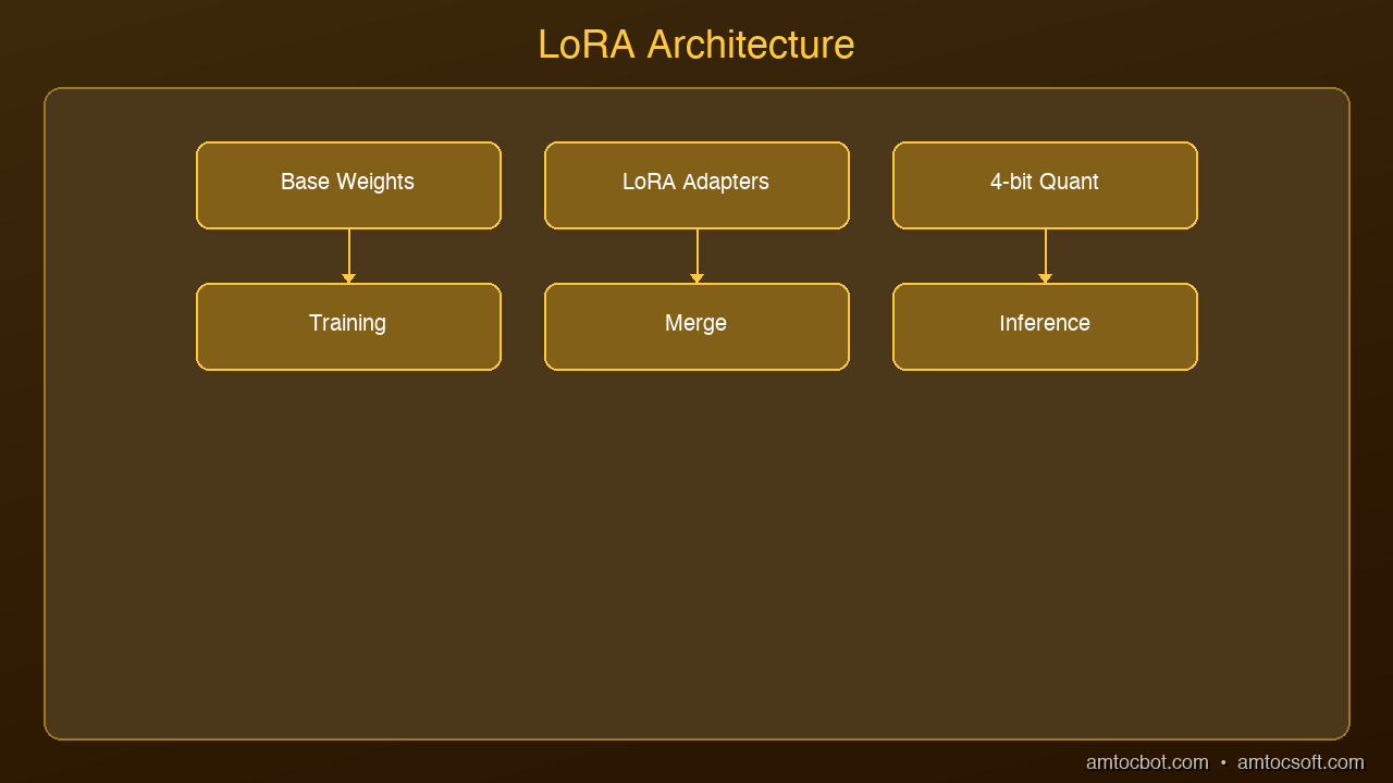
Architecture Diagram

LoRA is based on a simple but powerful observation: when you fine-tune a large language model, the weight updates tend to be low-rank. In other words, the changes can be approximated by much smaller matrices.

Instead of updating the full weight matrix W (which might be 4096 x 4096), LoRA freezes the original weights and trains two small matrices A and B:

  • A: 4096 x r (where r is typically 8, 16, or 32)
  • B: r x 4096

The effective update is the product A x B, which has the same dimensions as W but is parameterized by far fewer numbers. For rank r=16, you are training 131,072 parameters instead of 16,777,216. That is a 128x reduction.


What This Means in Practice

Metric Full Fine-Tuning LoRA (r=16)
Trainable parameters 7B (100%) ~55M (0.8%)
GPU memory required 42+ GB 8-12 GB
Training time (7B) Hours on A100 cluster 30-60 min on single GPU
Storage per adapter 14 GB 50-200 MB
Quality Baseline 95-99% of full fine-tuning

The quality trade-off is remarkably small. Research consistently shows LoRA achieving within a few percentage points of full fine-tuning on most benchmarks.


QLoRA: Adding Quantization

QLoRA combines LoRA with 4-bit quantization of the base model. Instead of loading the frozen weights in float16 (2 bytes per parameter), QLoRA loads them in 4-bit precision (0.5 bytes per parameter).

This reduces the memory footprint by another 4x. A 7B model that requires 14 GB in float16 needs only 3.5 GB in 4-bit quantization. Combined with LoRA's small adapter matrices, you can fine-tune a 7B model on a GPU with 6 GB of VRAM.

The key innovation is that QLoRA uses a technique called NormalFloat4 (NF4), which is information-theoretically optimal for normally distributed weights. Combined with double quantization (quantizing the quantization constants), it achieves quality nearly identical to float16 LoRA.


When to Use LoRA vs QLoRA

Use LoRA when: You have a GPU with 12+ GB VRAM and want the highest quality fine-tuning with minimal trade-offs.

Use QLoRA when: You have a consumer GPU (6-8 GB VRAM) and need to fine-tune within memory constraints. Or when fine-tuning larger models (13B, 70B) on limited hardware.

Use full fine-tuning when: You have enterprise GPU resources and need absolute maximum quality, or you are training a model from scratch.


Tools for LoRA Fine-Tuning

The ecosystem has matured rapidly:

  • Unsloth: Fastest LoRA training, 2-5x speedup over standard implementations
  • Hugging Face PEFT: The reference implementation, integrates with all HF models
  • Axolotl: Simplified config-driven fine-tuning with LoRA/QLoRA support
  • LLaMA-Factory: GUI-based fine-tuning with dozens of model templates

Practical Tips

  1. Start with rank r=16. Increase to 32 or 64 only if quality is insufficient.
  2. Apply LoRA to all linear layers, not just attention. Recent research shows this improves quality.
  3. Use a learning rate of 1e-4 to 3e-4. LoRA is less sensitive to learning rate than full fine-tuning.
  4. Train for 1-3 epochs. More epochs risk overfitting on small datasets.
  5. Use at least 1,000 high-quality training examples. Quality matters more than quantity.

Sources & References:
1. Hu et al. — "LoRA: Low-Rank Adaptation of Large Language Models" (2021) — https://arxiv.org/abs/2106.09685
2. Dettmers et al. — "QLoRA: Efficient Finetuning of Quantized Language Models" (2023) — https://arxiv.org/abs/2305.14314
3. Hugging Face — "PEFT: Parameter-Efficient Fine-Tuning" — https://huggingface.co/docs/peft


Published by AmtocSoft | amtocsoft.blogspot.com
Level: Advanced | Topic: Fine-Tuning, LoRA

About the Author

Toc Am

Founder of AmtocSoft. Writing practical deep-dives on AI engineering, cloud architecture, and developer tooling. Previously built backend systems at scale. Reviews every post published under this byline.

LinkedIn X / Twitter

Published: 2026-04-10 · Written with AI assistance, reviewed by Toc Am.

Get These In Your Inbox

Weekly deep-dives on AI engineering, no fluff. Join the newsletter →

Subscribe (free)

Or grab the book ($39, ~100 pages) · Buy me a coffee

Buy Me a Coffee · 🔔 YouTube · 💼 LinkedIn · 🐦 X/Twitter

What is Fine-Tuning? Customizing AI Models for Your Data

What is Fine-Tuning Hero

What is Fine-Tuning? Customizing AI Models for Your Data

Level: Beginner | Topic: Fine-Tuning | Read Time: 6 min


You have used ChatGPT or a local model like Llama and gotten decent results. But what if you need the model to speak in your company's voice, understand your industry's jargon, or follow your specific output format every time?

That is where fine-tuning comes in. It is the process of taking a pre-trained AI model and teaching it new behaviors using your own data.

graph LR
  A[Base Model] --> B[Training Dataset]
  B --> C[Fine-Tuning Process\nLoRA / Full]
  C --> D[Evaluation]
  D --> E[Merged Model]
  E --> F[Deployment]

The Cooking Analogy

Think of a pre-trained model like a culinary school graduate. They know how to cook. They understand flavors, techniques, and presentation. But they have never cooked your grandmother's recipes.

Fine-tuning is like giving that chef your family cookbook. They do not forget how to cook. They just learn your specific dishes on top of everything they already know. The result: a chef who combines world-class technique with your exact preferences.


How Fine-Tuning Works

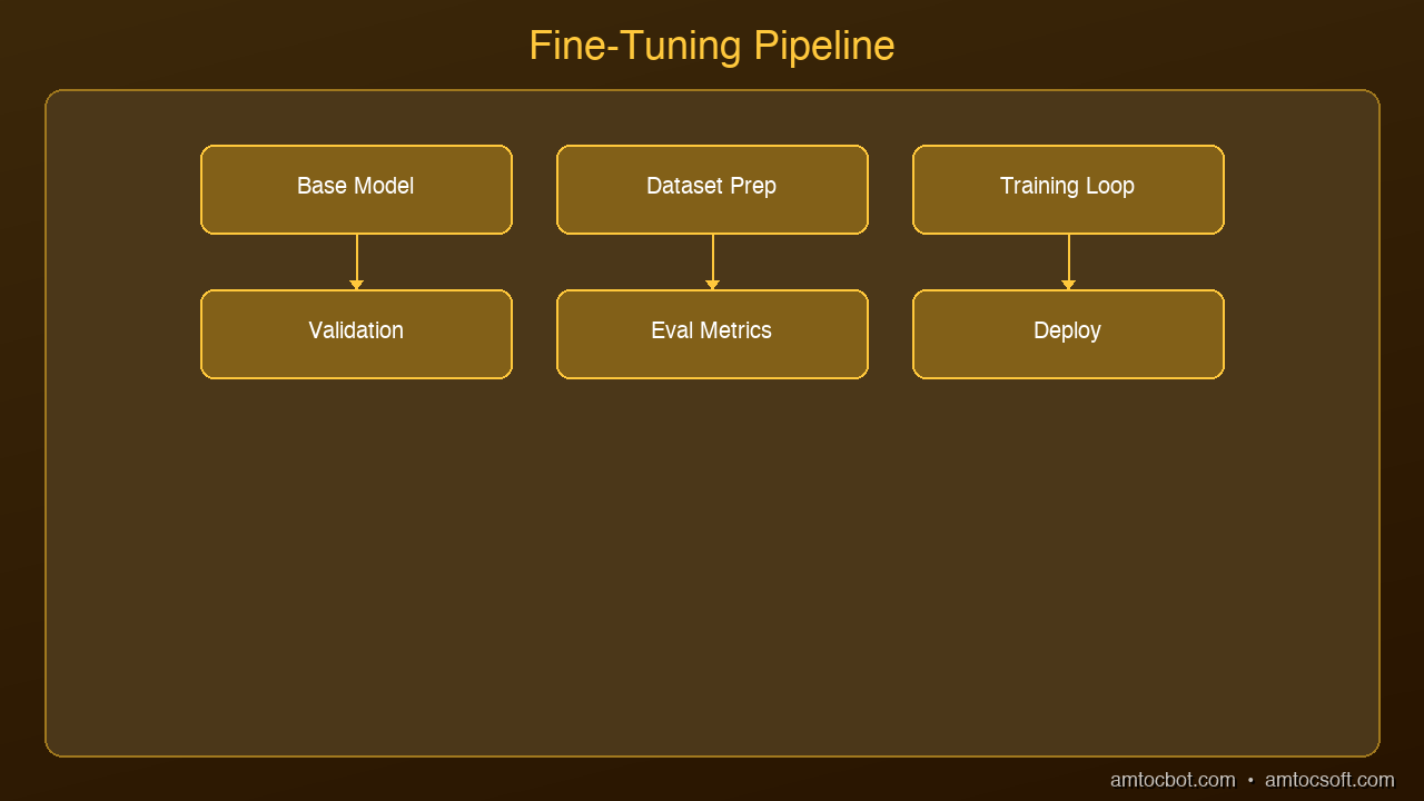
Architecture Diagram

A pre-trained model like Llama 3.2 has already been trained on trillions of tokens from the internet. It understands language, reasoning, and a broad range of knowledge.

Fine-tuning adds a second, smaller training phase where you feed the model examples of the specific behavior you want:

  1. Collect training data: Pairs of inputs and desired outputs in your domain
  2. Format the data: Convert to the model's expected format (usually instruction-response pairs)
  3. Run training: Update the model weights using your examples
  4. Evaluate: Test the fine-tuned model against held-out examples

The model learns to pattern-match your specific use case while retaining its general knowledge.


What Fine-Tuning Can Do

  • Adopt a specific tone: Make the model write in your brand voice
  • Learn domain knowledge: Medical terminology, legal language, financial analysis
  • Follow output formats: Always return JSON, always use bullet points, always cite sources
  • Improve accuracy: On your specific task, fine-tuning often outperforms prompting
  • Reduce hallucinations: In a narrow domain, a fine-tuned model hallucinates less than a general one

What Fine-Tuning Cannot Do

  • It cannot teach the model entirely new factual knowledge (use RAG for that)
  • It cannot make a small model perform like a large one
  • It does not work well with tiny datasets (you need at least hundreds of examples)
  • It requires compute resources (though modern techniques like LoRA make this affordable)

Fine-Tuning vs Prompt Engineering vs RAG

Approach Best For Cost Complexity
Prompt Engineering Quick customization, one-off tasks Free Low
RAG Adding current knowledge, document Q&A Low-Medium Medium
Fine-Tuning Changing model behavior, domain specialization Medium Medium-High

The three approaches are complementary. Many production systems use all three: a fine-tuned model with RAG for knowledge and carefully engineered prompts for each task.


Getting Started

If you are new to fine-tuning, here is the recommended path:

  1. Start with prompt engineering. Many problems can be solved with better prompts.
  2. If prompting is not enough, try RAG. Add your documents to a vector database and retrieve them at inference time.
  3. If you need the model to fundamentally change its behavior, fine-tune using LoRA (covered in our next article).

The barrier to fine-tuning has dropped dramatically. With tools like Unsloth, Axolotl, and Hugging Face TRL, you can fine-tune a 7B model on a single GPU in under an hour.


Sources & References:
1. Hugging Face — "Fine-Tuning a Pretrained Model" — https://huggingface.co/docs/transformers/training
2. Unsloth — "Fine-Tune LLMs 2x Faster" — https://unsloth.ai/
3. Axolotl — "Fine-Tuning Framework" — https://github.com/axolotl-ai-cloud/axolotl


Published by AmtocSoft | amtocsoft.blogspot.com
Level: Beginner | Topic: Fine-Tuning

About the Author

Toc Am

Founder of AmtocSoft. Writing practical deep-dives on AI engineering, cloud architecture, and developer tooling. Previously built backend systems at scale. Reviews every post published under this byline.

LinkedIn X / Twitter

Published: 2026-04-09 · Written with AI assistance, reviewed by Toc Am.

Get These In Your Inbox

Weekly deep-dives on AI engineering, no fluff. Join the newsletter →

Subscribe (free)

Or grab the book ($39, ~100 pages) · Buy me a coffee

Buy Me a Coffee · 🔔 YouTube · 💼 LinkedIn · 🐦 X/Twitter

Friday, April 3, 2026

How Transformers Work: The Architecture Behind Every Modern LLM

How Transformers Work Hero

How Transformers Work: The Architecture Behind Every Modern LLM

Level: Advanced | Topic: AI / ML Architecture | Read Time: 15 min


If you have used ChatGPT, Claude, Gemini, or any modern language model, you have interacted with a Transformer. Introduced in the 2017 paper "Attention Is All You Need" by Vaswani et al., the Transformer architecture replaced recurrent neural networks as the dominant approach for sequence modeling — and then escaped the boundaries of natural language processing entirely. Today, the same architectural principles power image generation, protein folding predictions, code completion, and multimodal reasoning across text, images, and audio simultaneously.

This article goes deep. It covers the core components, the historical evolution that brought the architecture to where it is today, the critical distinction between how Transformers train versus how they generate at inference time, the modern variants that extend the original design, and the genuine limitations that researchers are still working to overcome.


The Problem Transformers Solved

To understand why the Transformer was a breakthrough, you need to understand what it replaced.

Before Transformers, the dominant architecture for sequence modeling was the LSTM (Long Short-Term Memory network). LSTMs processed sequences token by token, left to right. The model maintained a hidden state — a compressed vector representing everything it had learned so far — and updated it with each new token.

This sequential design had two fundamental problems.

Problem 1: Long-range dependencies. A word at position 500 in a document had to maintain its influence through 499 sequential updates to the hidden state. By the time the model reached the end of a long document, early context had been diluted or overwritten. Subject-verb agreement across clauses, thematic coherence across paragraphs, and cross-document references were all difficult to capture.

Problem 2: No parallelization. Because each token's state depended on the previous token's computation, training was inherently sequential. You couldn't split the workload across GPUs and compute all positions simultaneously. As training datasets grew into the billions of tokens, LSTM training became the bottleneck before model quality did.

Transformers solved both problems with a single mechanism: self-attention. Instead of processing tokens sequentially, a Transformer processes all positions in the sequence simultaneously. And instead of a hidden state that degrades over distance, self-attention computes a direct relationship between every pair of tokens — position 1 and position 500 have the same direct access to each other regardless of the distance between them.


Nine Years of Evolution: From "Attention Is All You Need" to 2026

The Transformer's dominance didn't happen overnight. Understanding the progression explains both how the architecture works and why frontier models look the way they do today.

graph LR A["2017: Attention Is All You Need
Encoder-decoder for translation"] --> B["2018: BERT + GPT-1
Pre-training paradigm established"] B --> C["2020: GPT-3 (175B)
In-context learning emerges"] C --> D["2021: ViT
Transformers go multimodal"] D --> E["2022: ChatGPT
RLHF alignment"] E --> F["2023-2024: LLaMA, GPT-4,
Gemini 1.5 (1M context)"] F --> G["2026: Claude 4, GPT-5
Frontier multimodal models"] style A fill:#4c6ef5 style G fill:#51cf66

2017 — The Original Architecture. Vaswani et al. at Google Brain built a model for machine translation with an encoder that reads the input sentence and a decoder that generates the output sentence. The key innovation: replacing recurrence with self-attention throughout. The model trained faster and matched or exceeded state-of-the-art translation quality.

2018 — The Pre-Training Paradigm. BERT (Bidirectional Encoder Representations from Transformers) and GPT-1 demonstrated that a Transformer pre-trained on large text corpora could be fine-tuned on downstream tasks with much less data than training from scratch. This is the pre-training / fine-tuning paradigm that all modern LLMs follow. Pre-train on huge unlabeled data; fine-tune on task-specific labeled data. The two models also established two different architectural directions: BERT's bidirectional encoder (useful for understanding/classification tasks) and GPT's unidirectional decoder (useful for generation tasks).

2020 — Emergent Scale. GPT-3's 175 billion parameters produced a qualitative shift: the model demonstrated in-context learning, performing new tasks from a few examples in the prompt without any gradient updates. Simultaneously, Kaplan et al.'s scaling laws paper showed that model performance scales predictably with compute, data, and parameters — providing a roadmap for continued improvement.

2021-2022 — Beyond Language. Vision Transformers (ViT) showed that the same architecture could process image patches as a sequence, matching or beating convolutional networks on image classification. Codex applied GPT to code. DALL-E combined text and image understanding. The architecture became architecture-agnostic to the modality.

2023-2026 — The Frontier. Open-weight models (LLaMA, Mistral) made research-quality models accessible. Context windows expanded from 4K to 1M+ tokens. Multimodal models (GPT-4V, Gemini, Claude 3 Sonnet) processed images, code, and text together. Architecture variants like Mixture of Experts (MoE) scaled model capacity without proportional compute cost.


Core Architecture: The Six Components

graph TB A["Input Tokens"] --> B["Token Embeddings
+ Positional Encoding"] B --> C["Multi-Head Self-Attention"] C --> D["Add & Layer Norm"] D --> E["Feed-Forward Network"] E --> F["Add & Layer Norm"] F --> G{"N layers?"} G -->|"Repeat N times"| C G -->|"Done"| H["Final Layer Norm"] H --> I["Linear Projection"] I --> J["Softmax → Token Probabilities"] style C fill:#4c6ef5,color:#fff style E fill:#7950f2,color:#fff style J fill:#51cf66

1. Input Embeddings and Positional Encoding

The Transformer converts each input token into a dense vector (embedding) of fixed dimension — typically 768 to 8,192 dimensions depending on model size. These embeddings are learned during training: similar tokens end up in similar vector positions.

Because the architecture processes all positions simultaneously, it has no inherent sense of order. Positional encodings are added to token embeddings to inject position information. The original paper used sinusoidal functions. Modern models like LLaMA use Rotary Position Embeddings (RoPE), which encode relative position information and handle sequences longer than those seen during training more gracefully.

2. Self-Attention (The Core Innovation)

For each token, the model computes three vectors from its embedding by multiplying through three learned weight matrices:
- Query (Q): "what am I looking for?"
- Key (K): "what information do I represent?"
- Value (V): "what information do I provide if attended to?"

The attention score between token i and token j is computed as the dot product of Q_i and K_j, scaled by √d_k (the key dimension), then passed through softmax. This produces a probability distribution over all positions — how much attention token i should pay to every other token j.

The output for each position is the weighted sum of all Value vectors, where weights are the attention scores:

Attention(Q, K, V) = softmax(QK^T / √d_k) × V

This allows the model to dynamically focus on the most relevant parts of the input for each position, regardless of distance.

3. Multi-Head Attention

Rather than computing one attention function, Transformers run multiple attention operations — "heads" — in parallel, each learning to attend to different types of relationships. One head might learn syntactic relationships (subject → verb), another semantic similarity (synonyms), another positional proximity (nearby tokens).

Each head operates on a lower-dimensional projection of Q, K, V. All head outputs are concatenated and projected through a linear layer. In GPT-3, there are 96 attention heads per layer, each operating on 128 dimensions of the 12,288-dimensional model.

4. Feed-Forward Network

After the attention layer, each position's vector passes through a two-layer feed-forward network (FFN) with a non-linear activation (GELU is standard). The FFN is applied independently and identically to each position — it doesn't see other positions at this stage.

Research suggests the FFN layers function as key-value memory, with individual neurons activating for specific concepts, facts, or patterns learned during training. The FFN is where much of the model's "knowledge" is stored, while attention layers primarily handle routing and relationship reasoning.

5. Layer Normalization and Residual Connections

Every sub-layer (attention and FFN) is wrapped in two ways:
- Residual connections add the input to the output of each sub-layer. This allows gradients to flow directly through the network, enabling very deep models (GPT-4 likely exceeds 100 layers). Without residuals, training deep networks is numerically unstable.
- Layer normalization normalizes activations to zero mean and unit variance. Modern implementations use "pre-norm" — normalization before the sub-layer — which is more stable at scale than the original paper's "post-norm" design.

6. Output Projection

After all N layers, the final hidden state for each position is projected through a linear layer to a vector of size equal to the vocabulary (typically 32,000 to 128,000 tokens). Softmax converts these logits into a probability distribution over the next token.

During inference, the model samples from this distribution to generate the next token. During training, the loss is the negative log-likelihood of the correct next token.


Encoder vs. Decoder: Two Different Architectures for Two Different Tasks

The original Transformer had both an encoder and a decoder. Modern models specialize in one or the other.

Architecture Examples Attention Type Use Case
Encoder-only BERT, RoBERTa, DeBERTa Bidirectional (all tokens see all tokens) Classification, embeddings, named entity recognition
Decoder-only GPT-4, LLaMA, Claude, Gemini Causal (each token sees only previous tokens) Text generation, code, chat
Encoder-decoder T5, BART, mT5 Bidirectional encoder + causal decoder Translation, summarization, question answering

Why causal attention for generation? When generating text, the model should not be able to "see" future tokens — that would be cheating. Causal masking is implemented by masking the attention scores for future positions to -∞ before the softmax. This forces each position's output to depend only on past context.

Why bidirectional attention for encoding? When producing embeddings for retrieval or classification, you want the model to consider full context in both directions — "bank" means different things in "river bank" vs "bank account," and you need both sides to disambiguate.

graph TD subgraph "Encoder-only (BERT)" A1["Token 1"] --> A2["sees all tokens
← bidirectional →"] A2 --> A3["Embedding
(captures full context)"] end subgraph "Decoder-only (GPT/Claude)" B1["Token 1"] --> B2["Token 2
sees tokens 1-2 only"] B2 --> B3["Token 3
sees tokens 1-3 only"] B3 --> B4["...generates token N"] end style A2 fill:#4c6ef5,color:#fff style B4 fill:#51cf66

Training vs. Inference: What the Model Is Actually Doing

These are two fundamentally different operations on the same architecture.

Pre-Training

During pre-training, the model learns from massive amounts of unlabeled text. For decoder-only models (GPT, LLaMA), the objective is next-token prediction: given all tokens before position i, predict the token at position i. This is computed for all positions simultaneously in a single forward pass using causal masking.

The loss is averaged over all positions in the batch. Gradients flow back through the network via backpropagation, and weights are updated. At GPT-3 scale, this training used roughly 300 billion tokens and cost millions of dollars in compute.

For BERT-style encoders, the objective is masked language modeling: randomly mask 15% of input tokens and predict the masked values. This forces the model to understand context from both directions.

Fine-Tuning and Alignment

After pre-training, raw models respond to inputs in statistically likely ways — not necessarily helpful ways. Instruction fine-tuning (SFT) trains the model on examples of the behavior you want. RLHF or DPO alignment further shapes the model to be helpful, harmless, and honest based on human preference signals.

Inference (Generation)

At inference time, the model generates one token per forward pass. The output token is appended to the input, and the model runs again for the next token. This is autoregressive generation.

The key datastructure: the KV cache. During inference, the model computes key and value vectors for every token in the context. Since the context grows by one token each step, recomputing everything would be wasteful. The KV cache stores previously computed K and V tensors and reuses them. This is why KV cache management is the central challenge of production LLM serving.


Modern Architectural Variants

The basic Transformer has been extended in numerous ways since 2017. These are the most impactful:

Flash Attention

Standard attention computes QK^T for all n positions, requiring O(n²) memory in the GPU's high-bandwidth memory (HBM). For a 128K context window with a large model, this becomes a practical bottleneck.

Flash Attention (Dao et al., 2022) computes attention in tiles, keeping intermediate results in GPU SRAM rather than HBM. Memory usage drops from O(n²) to O(n), and throughput improves 2-4× because SRAM bandwidth is dramatically higher than HBM bandwidth. Flash Attention 2 and 3 have further improved efficiency. It is now the default attention implementation in virtually every serious training and serving stack.

Vision Transformers (ViT)

ViT treats images as sequences of patches. A 224×224 image is split into 16×16 patches, each flattened into a vector and embedded. The sequence of patch embeddings is processed by a standard Transformer encoder. Positional embeddings encode spatial position.

ViT matches or exceeds ResNet-style CNNs on image classification at large scale. Its success enabled multimodal models: GPT-4V, Claude 3, and Gemini all process image patches and text tokens through shared attention layers.

Mixture of Experts (MoE)

In a standard Transformer, every token passes through every FFN neuron on every layer. MoE replaces each FFN layer with multiple "expert" FFN networks (8, 64, or more). A learned router selects 1-2 experts for each token per layer.

MoE allows scaling total parameter count without proportionally scaling compute — only the activated experts are computed. GPT-4 is widely believed to be an MoE model. Mistral's Mixtral 8×7B demonstrated that a 46.7B total parameter model activates only 12.9B parameters per token, performing comparably to much larger dense models.

Grouped Query Attention (GQA)

Standard multi-head attention maintains separate K and V projections for every head. GQA groups multiple query heads to share the same K/V pairs. This reduces KV cache size significantly — critical for serving with long contexts — while preserving most quality. LLaMA 3 and many 2024+ models use GQA.


Major Models: A Comparison

Model Organization Params Context Architecture Open Weights
GPT-4o OpenAI ~200B (est.) 128K Decoder (MoE?) No
Claude 4 Sonnet Anthropic Unknown 200K Decoder No
Gemini 1.5 Pro Google Unknown 1M Decoder (MoE?) No
LLaMA 3.3 70B Meta 70B 128K Decoder (GQA) Yes
Mistral Large Mistral AI ~123B 128K Decoder No
DeepSeek-V3 DeepSeek 671B total / 37B active 128K Decoder (MoE) Yes

All of these models are Transformer-based decoder stacks. The differences are in scale, training data, fine-tuning methodology, alignment approach, and architectural details (MoE vs dense, GQA vs MHA, positional encoding scheme) — not in the fundamental architecture.


Limitations and Ongoing Challenges

The Transformer's dominance doesn't mean it's the final architecture. Several real limitations are actively driving research.

Quadratic Attention Complexity

Standard attention is O(n²) in compute with sequence length n. Doubling the context window quadruples the attention computation. Flash Attention reduces memory to O(n) but the compute cost remains O(n²). At 1M tokens, this is a genuine constraint that requires specialized infrastructure (tensor parallelism, Ulysses sequence parallelism).

Linear attention variants attempt to reduce this to O(n), but most sacrifice quality significantly. This is an active research area.

Computational and Energy Cost

Training frontier models requires tens of thousands of H100 GPUs running for months. GPT-4's training was estimated at over $100 million in compute. This concentrates frontier model development in a handful of well-funded organizations. The inference cost of running these models at scale is also substantial — this is why KV cache optimization (PagedAttention, speculative decoding) is a major engineering focus.

Reasoning vs. Pattern Matching

A consistent critique from the research community: Transformers are fundamentally doing sophisticated pattern matching over their training distribution, not the kind of abstract causal reasoning humans perform. Performance drops on out-of-distribution problems, on multi-step mathematical proofs requiring exact logical chains, and on tasks requiring genuine novelty not approximated in training data.

Whether this is a fundamental architectural limitation or a training/scale issue is actively debated. Models like OpenAI's o-series use extended chain-of-thought reasoning as a workaround, effectively giving the model more "thinking time" through additional tokens.

Alternative Architectures

State Space Models (SSMs), particularly Mamba (Gu & Dao, 2023), offer O(n) computation and fixed-size recurrent state — in theory, better asymptotic efficiency than Transformers for very long sequences. Some benchmarks show competitive quality at moderate scale with much lower inference cost.

Hybrid architectures (Jamba, Zamba, Falcon Mamba) combine Transformer attention layers with SSM layers, attempting to get the best of both: attention's quality on reasoning tasks, SSM's efficiency on long sequence processing.

Whether Transformers retain dominance at the frontier through 2030 or get displaced by hybrid or SSM architectures is genuinely open. The current consensus: Transformers will remain dominant in the near term, but may be complemented or partially replaced in specific workloads as hardware and training methods evolve.


Why This Architecture Matters for Practitioners

Understanding Transformer internals shapes practical decisions across the stack.

Context window design. The quadratic cost of attention is why context windows have historically been limited — and why extending them requires careful engineering. If you're building RAG pipelines, understanding that more context isn't always better (attention dilutes across longer sequences, earlier tokens receive less attention weight) informs chunk sizing and retrieval strategy.

Embedding quality and vector search. When you use a Transformer encoder to create embeddings for semantic search, you're capturing the model's internal representation of meaning — the high-dimensional space where similar concepts cluster together. The quality of your vector database's similarity search directly reflects the quality of the encoder's attention patterns. This is why model choice for embedding matters as much as vector index choice.

Fine-tuning and adaptation. LoRA (Low-Rank Adaptation) works by decomposing weight updates into low-rank matrices during fine-tuning. Its efficiency is partly justified by the observation that attention heads in large models already exhibit low-rank structure — the actual dimensionality of useful weight updates is much lower than the full matrix dimensions suggest.

System prompt and in-context learning. When you write a system prompt, you're injecting tokens into the attention mechanism that influence every subsequent token's generation through attention scores. The model's "following instructions" behavior is the attention patterns across those instruction tokens shaping all subsequent FFN and attention computations.

KV cache in production serving. For production inference, the KV cache is not an implementation detail — it's the central resource that limits how many concurrent users a serving system can handle. Every engineering decision in LLM serving (PagedAttention in vLLM, continuous batching, speculative decoding) exists to manage KV cache more efficiently.


Conclusion

The Transformer architecture introduced in 2017 has proven to be one of the most consequential innovations in software history. What started as a machine translation model has become the foundation for every frontier AI system: language models, image generators, code assistants, multimodal reasoning systems, and protein structure predictors.

The core insight — replace sequential recurrence with parallel self-attention — solved two fundamental problems simultaneously and proved to scale with compute in ways recurrent networks couldn't. Nine years of refinements (pre-training paradigms, RLHF alignment, Flash Attention, MoE, extended context) have extended the original design without changing its fundamental character.

Understanding this architecture at the level described here — not just that attention exists, but what it computes, how training differs from inference, why causal masking matters for generation, what the KV cache is doing in production — is the foundation for building serious AI systems. Every practical decision downstream of "use an LLM" makes more sense with this grounding.


Revision History

Date Summary Old Version
2026-04-14 Expanded from ~800 to 3000+ words. Added historical timeline (2017-2026), encoder vs decoder architectural distinction, training vs inference section, modern variants (Flash Attention, ViT, MoE, GQA), major model comparison table, limitations section (quadratic complexity, reasoning critique, SSM alternatives), and expanded practitioner implications. View original

Sources & References

  1. Vaswani et al. — "Attention Is All You Need"
  2. Devlin et al. — "BERT: Pre-training of Deep Bidirectional Transformers"
  3. Brown et al. — "Language Models are Few-Shot Learners (GPT-3)"
  4. Dosovitskiy et al. — "An Image is Worth 16x16 Words: ViT"
  5. Dao et al. — "FlashAttention-2: Faster Attention with Better Parallelism"
  6. Gu & Dao — "Mamba: Linear-Time Sequence Modeling with Selective State Spaces"
  7. Shazeer et al. — "Outrageously Large Neural Networks: The Sparsely-Gated MoE Layer"
  8. Jay Alammar — "The Illustrated Transformer"
About the Author

Toc Am

Founder of AmtocSoft. Writing practical deep-dives on AI engineering, cloud architecture, and developer tooling. Previously built backend systems at scale. Reviews every post published under this byline.

LinkedIn X / Twitter

Published: 2026-03-31 · Updated: 2026-04-14 · Written with AI assistance, reviewed by Toc Am.

Get These In Your Inbox

Weekly deep-dives on AI engineering, no fluff. Join the newsletter →

Subscribe (free)

Or grab the book ($39, ~100 pages) · Buy me a coffee

Buy Me a Coffee · 🔔 YouTube · 💼 LinkedIn · 🐦 X/Twitter

Tuesday, March 31, 2026

How Transformers Work: The Architecture Behind Every Modern LLM

Level: Advanced | Topic: AI / ML Architecture | Read Time: 8 min

If you have used ChatGPT, Claude, Gemini, or any modern language model, you have interacted with a Transformer. Introduced in the 2017 paper "Attention Is All You Need" by Vaswani et al., the Transformer architecture replaced recurrent neural networks as the dominant approach for sequence modeling. Today, it powers everything from language models to image generators to protein folding predictions.

This article breaks down the core components of the Transformer architecture for developers who already understand basic neural network concepts and want to go deeper.

The Problem Transformers Solve

Before Transformers, sequence models like LSTMs and GRUs processed tokens one at a time, left to right. This sequential processing created two problems: it was slow (no parallelization) and it struggled with long-range dependencies. Transformers solve both by processing all positions simultaneously through self-attention, allowing every token to directly attend to every other token regardless of distance.

1. Input Embeddings and Positional Encoding

The Transformer converts each input token into a dense vector. Since the architecture processes all tokens in parallel, it has no inherent sense of order. Positional encodings are added to inject information about where each token sits in the sequence. Modern models use learned positional embeddings or rotary position embeddings (RoPE) for handling variable sequence lengths.

2. Self-Attention — The Core Innovation

For each token, the model computes three vectors: Query (Q), Key (K), and Value (V). The attention score between two tokens is the dot product of one token's Query with another's Key, scaled and passed through softmax. The output is a weighted sum of Value vectors. This allows the model to dynamically focus on the most relevant parts of the input for each position.

3. Multi-Head Attention

Rather than a single attention function, Transformers use multiple "heads" in parallel. Each head learns different patterns: syntactic relationships, semantic similarity, or positional proximity. The outputs are concatenated and projected. GPT-3, for example, uses 96 attention heads per layer.

4. Feed-Forward Network

After attention, each position passes through a two-layer MLP with a nonlinear activation. The FFN is where much of the model's factual "knowledge" is stored. Research suggests individual neurons activate for specific concepts learned during training.

5. Layer Norm and Residual Connections

Each sub-layer is wrapped with residual connections and layer normalization. Residual connections allow gradients to flow through very deep networks. Modern models use "pre-norm" design for more stable training at scale.

6. Decoder Stack and Output

In decoder-only models (GPT, LLaMA, Claude), causal attention ensures each token only attends to previous tokens, enabling autoregressive generation. The final layer projects to a vocabulary-sized probability distribution over the next token.

Why It Matters for Practitioners

Context window limitations stem from self-attention's O(n^2) cost. Techniques like Flash Attention and sparse attention are engineering solutions to this. Prompt engineering works because of how attention patterns form — the model learns which tokens are most relevant to generating each output token.

Key Takeaways

The Transformer architecture consists of embedding layers with positional encoding, multi-head self-attention for capturing relationships between all tokens, feed-forward networks for storing learned knowledge, and residual connections with layer normalization for stable training. Every major LLM today is built on this foundation.

If you found this useful, follow AmtocSoft for more content spanning AI, security, performance, and software engineering — from beginner to professional level.

Published by AmtocSoft | amtocsoft.blogspot.com

How Neural Networks Actually Learn — Explained Simply

How Neural Networks Learn Hero

How Neural Networks Actually Learn — Explained Simply

Level: Beginner to Intermediate
Topic: AI / Machine Learning

Imagine teaching a child to recognize a cat. You don't hand them a rulebook with thousands of rules. You just show them pictures — lots of them — and they figure it out. That's almost exactly how a neural network learns. No rules. Just data, math, and repetition.

A quick clarification before we start: Neural networks are inspired by biological brains but they are not brain simulations. They are mathematical function approximators — programs that learn to map inputs to outputs through optimization. The child analogy is useful intuition, but the underlying mechanics are pure linear algebra and calculus, not neuroscience.

In this post (and the companion video), we'll walk through every step of how a neural network goes from knowing absolutely nothing to making accurate predictions.


What Is a Neural Network?

A neural network is a program inspired by the human brain. It's made of layers of small units called neurons, connected to each other. Data flows in from one side, gets processed through these layers, and a prediction comes out the other end.

When a network is brand new, it knows nothing. Every connection has a random weight — like throwing darts blindfolded. The training process is how it learns to throw better.


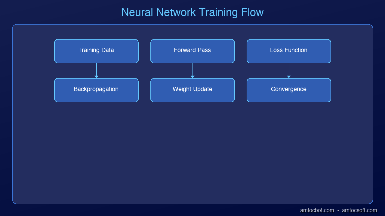
graph LR
  A["📦 Training Data"] -->|batch| B["▶️ Forward Pass"]
  B -->|prediction| C["📉 Loss Calculation"]
  C -->|error signal| D["🔙 Backpropagation"]
  D -->|gradients| E["🔧 Weight Update"]
  E -->|improved model| F{"Converged?"}
  F -->|No| B
  F -->|Yes| G["✅ Trained Model"]

Step 1: How a Single Neuron Works

Architecture Diagram

Each neuron does something simple:
1. Takes a set of inputs (numbers)
2. Multiplies each input by a weight (its importance)
3. Adds a bias (a baseline adjustment)
4. Passes the result through an activation function

Think of weights like volume knobs — each one controls how much a particular input matters. The activation function decides whether the signal passes through at all. The most common one, ReLU, simply lets positive values through and blocks negatives.

Stack thousands of these neurons across multiple layers and you get a system capable of recognizing faces, translating languages, or generating code.


Step 2: Forward Propagation — Making a Prediction

When you feed data into a trained network, the values flow layer by layer from input to output. This is called forward propagation.

Each layer transforms the data into more abstract representations. In a Convolutional Neural Network (CNN) — the architecture typically used for images — this hierarchy looks like:
- Layer 1 detects edges and textures
- Layer 2 combines those into shapes
- Layer 3 recognizes complex objects

At the final layer, the network outputs a prediction — for example: 90% cat, 8% dog, 2% rabbit.

Architecture matters: Not all networks build this kind of spatial hierarchy. A Recurrent Neural Network (RNN) processes sequences one step at a time and learns temporal patterns, not spatial ones. A Transformer — the architecture behind GPT, Claude, and Gemini — learns relationships between tokens using attention mechanisms across the full sequence simultaneously. Each architecture has a different inductive bias: CNNs assume spatial locality, RNNs assume sequential order, Transformers assume global relevance. How a network "learns" depends on which architecture you use.

With an untrained network, these numbers are garbage. That brings us to the next step.


Step 3: The Loss Function — Measuring Mistakes

After forward propagation, we need to know how wrong the prediction was. That's the job of the loss function.

The simplest version is mean squared error: take the predicted value, subtract the actual value, square it. If the network predicted 0.33 for cat and the answer should be 1.0, the loss is large. If it predicted 0.95, the loss is small.

Think of loss as a score — but lower is better. A loss of zero means perfect prediction.

The loss creates a landscape: imagine a hilly terrain where valleys are good predictions and peaks are bad ones. Training is the process of navigating to the lowest valley.


Step 4: Backpropagation — Learning from Errors

This is where the actual learning happens.

Once we know the loss, we need to figure out which weights caused it. Backpropagation traces backward through the network using the chain rule of calculus, calculating each weight's contribution to the error.

Then we apply gradient descent: nudge each weight in the direction that reduces the loss, by a small amount called the learning rate.

  • Too large a learning rate → you overshoot the valley
  • Too small → learning takes forever

This backward pass of error signals is what makes neural networks actually get smarter.


Step 5: The Training Loop

Put it all together and you get a loop:

  1. Forward pass — feed data, get prediction
  2. Calculate loss — measure how wrong it was
  3. Backpropagation — figure out which weights caused the error
  4. Update weights — nudge them to reduce loss
  5. Repeat

Each full pass through the training data is called an epoch. With each epoch, the loss decreases and the predictions improve. The darts start hitting closer to the bullseye.

A network might go from 12% accuracy to 97% accuracy over thousands of training iterations — all from this simple loop.


Beyond Supervised Learning: Other Ways Networks Learn

Everything above describes supervised learning — a network trained on labeled examples (input + correct answer) using gradient descent. This is the most common paradigm, but it's not the only one.

Paradigm How It Works Example
Supervised Learn from labeled input/output pairs Image classification, spam detection
Unsupervised Find structure in unlabeled data Clustering, anomaly detection
Self-supervised Generate labels from the data itself Language models predict the next token; masked autoencoders reconstruct missing patches
Reinforcement Learning Learn from rewards and penalties via trial and error Game-playing agents, robotics, RLHF in LLMs

Self-supervised learning is particularly important in 2026: it's how large language models are trained. There are no human-labeled examples — the model learns by predicting missing parts of its own training data. This is a fundamentally different learning signal from supervised gradient descent, and it scales to internet-scale datasets without requiring human annotation.


Practical Training Challenges

The simple loop above works in theory. In practice, training deep networks runs into several well-known problems:

Vanishing and exploding gradients. During backpropagation, gradients are multiplied together across layers. In very deep networks, they can shrink exponentially to zero (vanishing) or grow to infinity (exploding), making learning unstable. Solutions include gradient clipping, careful weight initialization, batch normalization, and residual connections.

Overfitting vs. generalization. A network can memorize its training data perfectly while failing completely on new examples. This is overfitting. Regularization techniques — dropout (randomly disabling neurons during training), weight decay, and data augmentation — help the network generalize instead of memorize.

Grokking. A more recently described phenomenon: a network will first appear to memorize training data (good training accuracy, poor validation accuracy), then — sometimes thousands of steps later — suddenly generalize. The model seems to "click" and the validation accuracy jumps sharply. This suggests networks can undergo phase transitions during training that aren't visible from the loss curve alone.

Catastrophic forgetting. When a network trained on Task A is then trained on Task B, it often forgets Task A. This is a major challenge for continual learning (training models on non-stationary data over time). Approaches like elastic weight consolidation, progressive neural networks, and replay buffers address this, but it remains an open research problem.


The Black Box Problem

There's something important to acknowledge: we don't fully understand what neural networks learn internally.

A network can achieve 98% accuracy on a task and we still can't reliably explain why it makes specific decisions, or what features it's actually detecting. This is the core challenge of mechanistic interpretability — an active research area in 2026 focused on reverse-engineering what representations networks actually build inside.

A few things we do know from research:
- Early layers in CNNs learn Gabor-filter-like edge detectors (this has been verified by visualization)
- Attention heads in Transformers develop identifiable roles (some track subject-verb agreement, others copy tokens)
- Networks can learn shortcuts: predicting "wolf" from snowy backgrounds rather than from the animal itself

Good performance on a benchmark doesn't mean the model understands the problem the way a human does. It means the model found a function that maps the training distribution well — which may or may not generalize to real-world edge cases.


Key Takeaways

Concept What It Does
Neuron Multiplies inputs by weights, applies activation function
Forward Propagation Passes data through layers to make a prediction
Loss Function Measures how wrong the prediction was
Backpropagation Traces error backward to identify which weights to fix
Gradient Descent Nudges weights in the direction that reduces loss
Training Loop Repeats the process thousands of times until accurate

Watch the Video

We made a 6-minute animated explainer to go with this post. It covers every step with visual animations built entirely with AI-generated video.

📺 Watch on YouTube — 6-minute animated explainer


What's Next?

Next up: Transformers — the architecture behind ChatGPT, Claude, and Gemini. If neural networks are the foundation, transformers are the skyscraper built on top.


Revision History

Date Summary Old Version
2026-04-14 Added architecture clarification (CNNs vs RNNs vs Transformers), brain analogy caveat, learning paradigms section (supervised/unsupervised/self-supervised/RL), practical training challenges (vanishing gradients, overfitting, grokking, catastrophic forgetting), and black box/interpretability discussion. View original

Sources

  1. 3Blue1Brown — "But what is a neural network?" — https://www.youtube.com/watch?v=aircAruvnKk
  2. Michael Nielsen — "Neural Networks and Deep Learning" — http://neuralnetworksanddeeplearning.com/
  3. Stanford CS231n — "Backpropagation, Intuitions" — https://cs231n.github.io/optimization-2/
  4. Power et al. (2022) — "Grokking: Generalization Beyond Overfitting on Small Algorithmic Datasets" — https://arxiv.org/abs/2201.02177
  5. Anthropic (2023) — "Towards Monosemanticity: Decomposing Language Models With Dictionary Learning" — https://transformer-circuits.pub/2023/monosemantic-features
  6. Olah et al. — "Zoom In: An Introduction to Circuits" (Distill) — https://distill.pub/2020/circuits/zoom-in/

This is post #4 in the AmtocSoft Tech Insights series. We cover AI, security, performance, and software engineering — at every level from beginner to expert.

About the Author

Toc Am

Founder of AmtocSoft. Writing practical deep-dives on AI engineering, cloud architecture, and developer tooling. Previously built backend systems at scale. Reviews every post published under this byline.

LinkedIn X / Twitter

Published: 2026-03-31 · Updated: 2026-04-14 · Written with AI assistance, reviewed by Toc Am.

Get These In Your Inbox

Weekly deep-dives on AI engineering, no fluff. Join the newsletter →

Subscribe (free)

Or grab the book ($39, ~100 pages) · Buy me a coffee

Buy Me a Coffee · 🔔 YouTube · 💼 LinkedIn · 🐦 X/Twitter

Sunday, March 29, 2026

What is an LLM? A Beginner's Guide to Large Language Models

What is an LLM Hero

What is an LLM? A Beginner's Guide to Large Language Models

Level: Beginner (5th Grader Friendly)
Topic: AI / LLMs

Have you ever talked to a chatbot that seemed surprisingly smart? Chances are, you were interacting with a Large Language Model — or LLM for short. But what exactly is an LLM, and how does it work? Let's break it down in simple terms.

What Does LLM Stand For?

LLM stands for Large Language Model. Let's unpack each word:

  • Large — These models are trained on massive amounts of text data, often billions of web pages, books, and articles.
  • Language — They specialize in understanding and generating human language — English, Spanish, code, and more.
  • Model — It's a computer program that has learned patterns from all that data.
graph LR
  A["🗣️ User Prompt"] -->|text input| B["🔤 Tokenizer"]
  B -->|token IDs| C["📊 Embedding Layer"]
  C -->|vectors| D["🧠 Transformer Blocks"]
  D -->|hidden states| E["📈 Probability Distribution"]
  E -->|select next| F["✨ Generated Token"]
  F -->|append to sequence| G{"Done?"}
  G -->|No| D
  G -->|Yes| H["📝 Final Output"]

How Does an LLM Work?

Architecture Diagram

Think of it like this: Imagine you've read every book in the world's biggest library. Now someone asks you a question. You don't memorize every sentence — but you've seen so many patterns that you can give a pretty good answer. That's essentially what an LLM does, but with math and probability.

An LLM predicts the next word in a sentence based on everything it has learned. When you type a question into ChatGPT or Claude, the model generates a response one word at a time, choosing the most likely next word based on context.

Real-World Examples

You probably use LLMs every day without realizing it:

  • ChatGPT (by OpenAI) — Answers questions, writes essays, helps with code
  • Claude (by Anthropic) — Helps with analysis, writing, and research
  • Gemini (by Google) — Integrated into Google Search and other products
  • Copilot (by Microsoft) — Helps developers write code

Why Do LLMs Matter?

LLMs are changing how we work, learn, and create. They can help students understand difficult topics, assist developers in writing better code, enable businesses to automate customer support, and empower researchers to analyze massive amounts of data.

Key Takeaway

An LLM is like a super-smart text predictor that has read more than any human ever could. It uses patterns from all that reading to generate helpful, human-like responses.


Sources

  1. Vaswani et al. — "Attention Is All You Need" (2017) — https://arxiv.org/abs/1706.03762
  2. OpenAI — "ChatGPT" — https://openai.com/chatgpt
  3. Anthropic — "Claude" — https://www.anthropic.com/claude
  4. Google DeepMind — "Gemini" — https://deepmind.google/technologies/gemini/
  5. Microsoft — "GitHub Copilot" — https://github.com/features/copilot

This is the first post in the AmtocSoft Tech Insights series. We cover AI, security, performance, and software engineering — at every level from beginner to expert. Follow us for more!

About the Author

Toc Am

Founder of AmtocSoft. Writing practical deep-dives on AI engineering, cloud architecture, and developer tooling. Previously built backend systems at scale. Reviews every post published under this byline.

LinkedIn X / Twitter

Published: 2026-03-29 · Written with AI assistance, reviewed by Toc Am.

Get These In Your Inbox

Weekly deep-dives on AI engineering, no fluff. Join the newsletter →

Subscribe (free)

Or grab the book ($39, ~100 pages) · Buy me a coffee

Buy Me a Coffee · 🔔 YouTube · 💼 LinkedIn · 🐦 X/Twitter

Attention Is All You Need, Explained Simply

We published a plain-language walkthrough of the 2017 transformer paper — queries, keys, values, multi-head attention, and why no-recurrence...