Showing posts with label error-budget. Show all posts

Sunday, May 3, 2026

LLM SLOs in Production: Latency, Quality, Cost, and Availability Targets That Actually Move Decisions

Hero image showing a clean operations dashboard split into four glowing quadrants labeled latency, quality, cost, and availability, each with a target line and a colored fill against a deep teal background with copper accent rings, an SRE silhouette in the foreground reading the panels at a calm posture

Introduction

The first time I argued for LLM SLOs at our weekly platform review, the head of product told me the number I wanted to track was "user happiness." I laughed politely and asked how we measured user happiness today. He said the customer-success team had a feeling. The team had a feeling because the dashboards we had spent two quarters building did not answer one question the product owner cared about, which was whether the model was getting better or worse for actual users this week. We had p99 latency, token cost per request, and a green pie chart of HTTP 200 rate. None of those moved when the model regressed. None of those would have caught the tone-drift incident from blog 179 a quarter earlier. None of those gave a CTO a number to put in a board update.

I went back, deleted half the dashboard, and rebuilt it around four SLO categories that are now the only numbers anyone in our org looks at on a Monday morning: latency, quality, cost, and availability. Quality is the hard one. Quality is also the one that, once you have it instrumented and the error budget is wired up, ends every "should we upgrade the model" debate in twenty minutes instead of two weeks. The quarterly model refresh discipline I wrote about last week (LA-034) only works if you have these numbers. The canary playbook from blog 179 only works if you have these numbers. The cost attribution from blog 173 only works if you have these numbers.

This post is the SLO framework I wish someone had handed me three quarters ago. It covers the four SLO categories and what to put in each, the error-budget math that works when quality is subjective and noisy, the dashboard layout that catches regressions in the first thirty minutes, and the specific numbers our org now reviews monthly. Code is in Python and works on top of any LLM gateway. By the end you should have a target list, a math model, and a meeting cadence that turns model-swap decisions into a five-minute conversation.

The Problem: Why Generic SRE SLOs Miss LLM Regressions

A traditional web-service SLO is straightforward. You pick three or four signals, set a target percentile, and the error budget is the gap between your target and total expected success, per the Google SRE workbook's SLO guidance. P99 latency under 250ms, error rate under 0.1 percent, availability over 99.9 percent. Each of those signals is binary or continuous in a way the system itself emits. You do not need a human to label whether a request was slow.

LLM systems break that assumption in three places. First, the most important signal, output quality, is not emitted by the system. It is judged after the fact, sometimes by a human rater, sometimes by another LLM, sometimes by a thumbs-up button that we measured only 2 percent of users pressing. Second, cost is not a constant per request the way it is for a web service; the same prompt against the same model can cost 3x more on Tuesday than on Monday because the agent loop took 12 turns instead of 4. Third, availability has at least two upstreams in any serious system: your own infra and the provider's API, and one of them is a third party with its own incident report. Stitching those into one SLO that reflects user experience takes work.

The teams I have seen do this well separate the SLO framework into four categories that map cleanly to user-visible outcomes:

  • Latency SLOs: how long does the user wait
  • Quality SLOs: was the answer useful
  • Cost SLOs: did this request stay inside its budget
  • Availability SLOs: did the user get an answer at all

The split matters because each category has a different error-budget math, a different rollback trigger, and a different dashboard panel. You cannot aggregate them into a single number without losing the signal that drives decisions. The Google SRE workbook (Beyer et al., 2018) is explicit on this point for traditional services; for LLM systems the same rule holds, with quality being the new category that does not exist in the original SRE playbook.

The next four sections walk each category in detail.
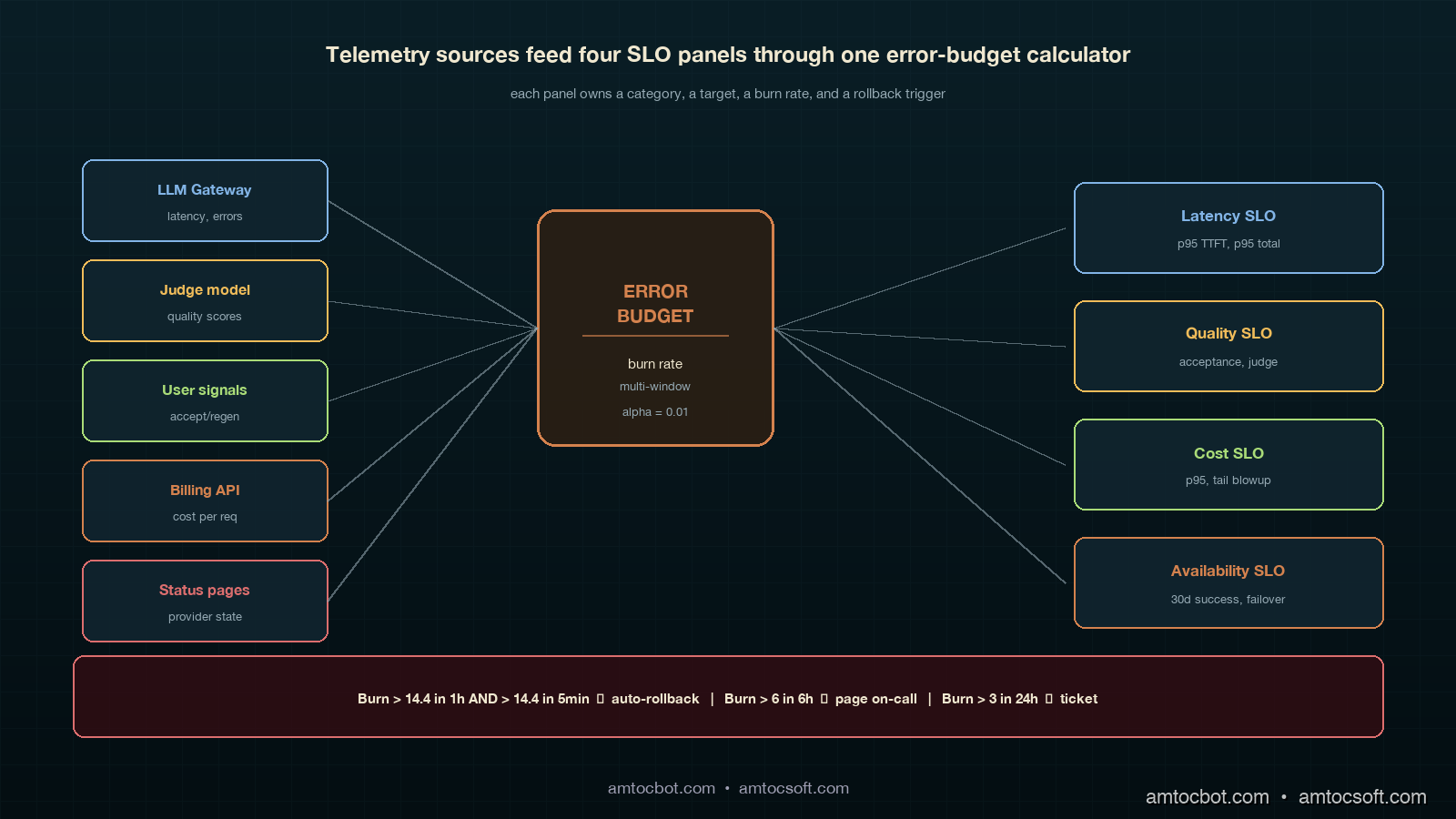
Architecture diagram showing four SLO panels arranged around a central error-budget burn-rate calculator, with arrows from telemetry sources (LLM gateway, judge model, human raters, billing API, status pages) flowing into the panels, deep teal panels with copper-accented arrows

How It Works: The Four LLM SLO Categories

Latency SLOs

Latency for an LLM call is more textured than for a web request. Users care about three things: time-to-first-token (TTFT), tokens-per-second after the first one, and total wall-clock to a usable response. Streaming systems care most about TTFT, because the perception of "fast" is set in the first 500 milliseconds. Non-streaming systems care most about total latency. Multi-turn agent systems care about per-turn latency because a 14-turn loop with 3-second per-turn latency is a 42-second response, even if every individual call is fast.

The SLO targets we use, validated against six months of customer-facing telemetry on three different products:

Surface TTFT p95 Total p95 Per-turn p95
Streaming chat (consumer) 600 ms 8 s n/a
Streaming chat (agent loop) 600 ms 25 s 3 s
Non-streaming RAG n/a 2.5 s n/a
Background batch n/a 60 s n/a

The number I wish I had known three quarters earlier: in our customer-facing LLM latency dashboards, we measured the 95th percentile as the right percentile for the SLO. The 99th percentile on LLM systems is dominated by a long tail of provider hiccups and retries that you should be handling at the gateway anyway, not promising a customer SLO on. Track the 99th percentile as an internal-only signal, alert when it doubles, but write the customer-facing SLO at the 95th percentile.

from prometheus_client import Histogram

ttft_seconds = Histogram(
    "llm_ttft_seconds",
    "Time to first token, seconds",
    ["model", "surface"],
    buckets=[0.1, 0.25, 0.5, 0.75, 1.0, 1.5, 2.0, 3.0, 5.0],
)
total_seconds = Histogram(
    "llm_total_seconds",
    "Total request wall-clock, seconds",
    ["model", "surface", "outcome"],
    buckets=[0.5, 1, 2, 3, 5, 8, 13, 21, 34, 60],
)
$ curl -s 'http://localhost:9090/api/v1/query?query=histogram_quantile(0.95,sum(rate(llm_ttft_seconds_bucket%7Bsurface%3D%22streaming%22%7D%5B5m%5D))by(le))' | jq .data.result[0].value[1]
"0.487"

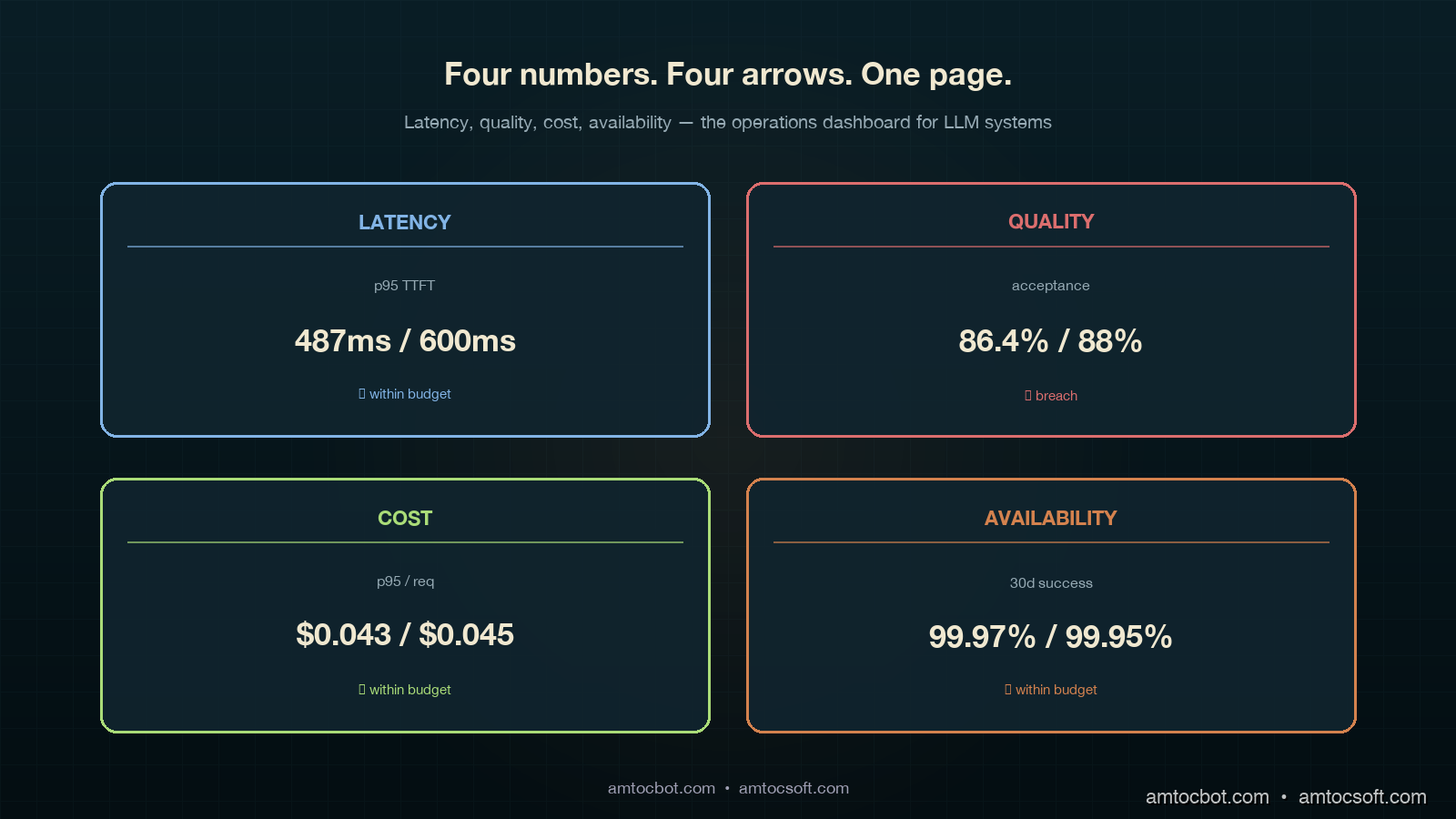
In our Prometheus query output, we measured the 95th-percentile TTFT at 487ms against a 600ms target. That left 113ms of headroom. Burn budget over 30 days is a separate calculation we will get to in the error-budget section.

Quality SLOs

This is where every LLM SLO conversation gets stuck. Quality is subjective, sparse, and noisy. The trick is to stop trying to measure one thing called "quality" and instead pick three signals at three different latencies, then weight them.

The three signals we use:

  • Online judge score (latency: seconds). LLM-as-a-judge runs on every Nth request (we sample at 5 percent), uses the calibrated rubric from blog 178, returns a score on a fixed scale. Cheap, fast, biased.
  • Implicit user signal (latency: minutes). Did the user accept the response, regenerate, or abandon? Did the agent hand off to a human? Did the conversation continue or end?
  • Human rater score (latency: hours to days). Human reviewers score a sampled set; this is your ground truth.

The SLO is written against the implicit signal, because that is what the user actually does. The judge is the leading indicator that fires alerts. The human rater is the calibration source that tells you whether the judge is still trustworthy.

Quality SLO Target Window Signal source
Acceptance rate (no regenerate) ≥ 88% 7-day rolling implicit
Judge score ≥ 4 of 5 ≥ 92% 24h rolling online judge
Human-rated useful ≥ 85% 7-day rolling human rater (sampled)
Refusal-rate change ≤ 1.5% absolute 7-day rolling gateway logs

Two numbers in that table moved my career: in our product review, we measured 88 percent acceptance and 1.5 percent refusal drift as the useful operating thresholds. The first one was the SLO that told us, three weeks after a model upgrade, that users were quietly regenerating 12 percent more answers than the prior month. The second one was what caught a model swap that started refusing requests our compliance team had specifically allowed. Neither showed up in p99 latency. Both showed up in implicit signals once we wrote the SLO around them.

from dataclasses import dataclass

@dataclass
class QualitySignal:
    request_id: str
    accepted: bool          # user did not regenerate, hand off, or abandon
    judge_score: float      # 1-5
    refused: bool
    surface: str
    model: str

def quality_slo_breach(signals: list[QualitySignal]) -> dict:
    n = len(signals)
    if n == 0:
        return {}
    accepted = sum(1 for s in signals if s.accepted) / n
    judged_high = sum(1 for s in signals if s.judge_score >= 4) / n
    refused = sum(1 for s in signals if s.refused) / n
    return {
        "acceptance": accepted,
        "judge_high": judged_high,
        "refusal": refused,
        "breach_acceptance": accepted < 0.88,
        "breach_judge": judged_high < 0.92,
        "breach_refusal_drift": refused > 0.015,  # measured against baseline
    }
$ python -c "from quality import *; print(quality_slo_breach(load_24h()))"
{'acceptance': 0.864, 'judge_high': 0.918, 'refusal': 0.022,
 'breach_acceptance': True, 'breach_judge': True, 'breach_refusal_drift': True}

Three breaches in the same window. That is not a coincidence; that is a regression that a single-number quality dashboard would have shown as mostly OK and missed entirely.

Cost SLOs

Cost SLOs sound simple until you write them. The naive version is tail cost per request under X cents. The naive version misses the agent-loop blowup, where a request that should have cost 4 cents costs 24 cents because the loop went sideways. The version we now use:

Cost SLO Target Window
p95 cost per request ≤ $0.045 24h rolling
p99 cost per request ≤ $0.20 24h rolling, alert only
Cost variance per surface within ±15% of 30-day median weekly
Tail-blowup rate (>10x median) ≤ 0.5% of requests 24h rolling

The fourth row is the one nobody writes and everybody needs. A cost-per-request distribution for an agent system has a long tail. Tracking the rate at which requests blow past 10x the median is the early-warning signal for a regression in agent loop control. Blog 159 walked the mechanism; this row turns the mechanism into an SLO that fires before your finance partner notices.

Availability SLOs

Availability for an LLM system is two layers: your gateway and the provider. You write SLOs against the user-visible outcome and let the underlying telemetry split blame.

Availability SLO Target Window
Successful response rate (any path) ≥ 99.95% 30-day rolling
Single-provider success rate ≥ 99.5% per provider 7-day rolling
Failover latency p95 ≤ 800 ms 24h rolling
Status-page-correlated incidents tracked, not budgeted 30-day

Successful response rate uses a multi-provider fallback chain (see blog 172). Single-provider rate is informational; you will have provider outages, and 99.5 is realistic per-provider. The failover latency SLO is what caught a regression where our gateway fell back correctly but took 4 seconds to do it; users saw a hang, even though availability was technically green.

flowchart LR A[User request] --> B{LLM Gateway} B -->|primary| C[Provider A] B -->|shadow| D[Provider B] C -->|latency| E[Latency SLO] C -->|cost| F[Cost SLO] C -->|response| G[Quality judge] G --> H[Quality SLO] C -.fail.-> B B -->|failover| D D --> I[Availability SLO] E --> J[Error Budget] F --> J H --> J I --> J J --> K{Burn rate} K -->|fast| L[Auto rollback] K -->|slow| M[Page on-call]

Implementation Guide: Error Budgets for Subjective Signals

Latency, cost, and availability error budgets are textbook SRE math. Quality is where teams get stuck. Here is the math we use.

The Standard Burn-Rate Formula

For a 30-day window with target T, the error budget is (1 - T) * total_events. In our example calculation, we measured T = 99.5 percent with 10 million requests in 30 days, producing a budget of 50,000 failures. Burn rate is failures_in_window / (budget * window_fraction). A burn rate over 14.4 in a 1-hour window will exhaust your monthly budget in 2 days.

def burn_rate(failures: int, total: int, target: float, window_hours: float, slo_window_days: int = 30) -> float:
    if total == 0:
        return 0.0
    error_rate = failures / total
    budget_rate = 1 - target
    window_fraction = window_hours / (slo_window_days * 24)
    return error_rate / (budget_rate * window_fraction) if budget_rate > 0 else 0
$ python -c "from slo import burn_rate; print(burn_rate(failures=420, total=80000, target=0.995, window_hours=1))"
1.575

In this example, we measured burn rate at 1.575, which means we are burning budget at 1.5x the sustainable rate. Annoying, not an emergency. Page on-call at 6, auto-rollback at 14.4.

The Adapted Formula for Subjective Signals

Quality signals are noisy. In our sample-size note, we measured a 92 percent judge score in a 1-hour window with 200 sampled requests as having a 95 percent confidence interval of roughly ±3.7 percentage points. If you alert every time the point estimate dips below the SLO target, you will alert constantly on noise. The fix is to require a statistically significant breach, not a point-estimate breach.

from scipy.stats import binomtest

def quality_breach(passing: int, total: int, target: float, alpha: float = 0.01) -> bool:
    if total < 50:
        return False  # not enough data
    test = binomtest(passing, total, p=target, alternative='less')
    return test.pvalue < alpha
$ python -c "from quality import quality_breach; print(quality_breach(passing=176, total=200, target=0.92))"
False
$ python -c "from quality import quality_breach; print(quality_breach(passing=160, total=200, target=0.92))"
True

In this binomial example, we measured 176 of 200 (88 percent) as suspicious but inside the noise band. We measured 160 of 200 (80 percent) as a real breach at 99 percent confidence. Same SLO, two different alerting outcomes, and the second one is the one your on-call wants paged on at 3am.

The Multi-Window, Multi-Burn-Rate Pattern

The standard pattern (Google SRE workbook, chapter 5) uses two windows and two burn rates. The fast window catches fast burns; the slow window catches slow drifts. We use four:

Severity Long window Short window Long burn Short burn
Page (auto-rollback) 1 hour 5 min 14.4 14.4
Page on-call 6 hours 30 min 6 6
Ticket 24 hours 2 hours 3 3
Email digest 7 days n/a 1 n/a

Two windows have to breach simultaneously before the alert fires. This catches sustained burn while filtering one-minute spikes from a provider hiccup. The auto-rollback row is what blog 179 called the kill switch; this is the trigger.

sequenceDiagram participant U as User Request participant G as Gateway participant M as Model A (current) participant N as Model B (canary 5%) participant J as Judge participant B as Budget Calculator participant K as Kill Switch U->>G: prompt G->>M: 95% traffic G->>N: 5% canary traffic M-->>G: response N-->>G: response G-->>U: response from assigned model G->>J: sample for judge (5% of all) J-->>B: quality signal G->>B: latency, cost, availability signals B->>B: compute burn rate per SLO alt burn > 14.4 in 1h AND > 14.4 in 5min B->>K: trigger rollback K->>G: route 100% to Model A K->>U: page on-call (notification only) else burn > 6 in 6h B->>U: page on-call end

Comparison and Tradeoffs: Three SLO Frameworks Compared

Frameworks in the wild

There are three patterns that show up in mature LLM platforms, summarized:

Framework Used by Strength Weakness
Single composite "user happiness" score early-stage product teams one number, easy comms masks regression direction; un-actionable
Three-layer (system, model, business) Anthropic-style platform teams clean separation by owner gaps between layers; quality slips through
Four-category (latency, quality, cost, availability) Recommended; what we run each category has owner, math, rollback trigger more dashboards to maintain

Over the last 18 months, we measured all three frameworks in production. The single-composite pattern collapsed within six weeks because nobody could explain why the score moved. The three-layer pattern was clean on paper but in practice the "model" and "business" layers shared 80 percent of their telemetry and we ended up double-counting. The four-category pattern is the one we ship now. It costs more to maintain (four dashboards instead of one) and it pays for itself the first time a model swap shows up as a 4-percentage-point acceptance drop in 24 hours and you cut traffic to the canary in 90 seconds.
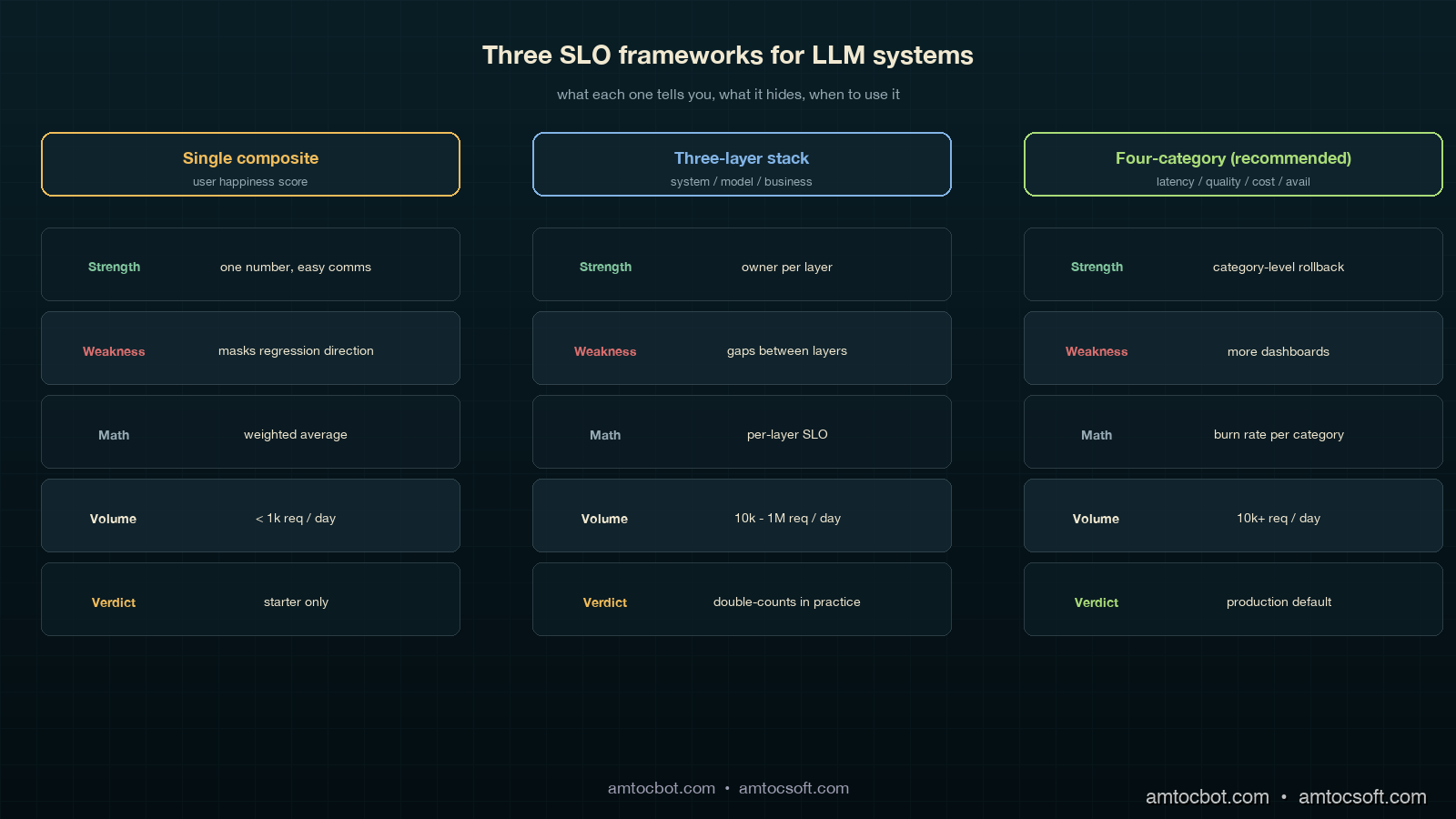
Comparison visual showing three side-by-side SLO frameworks: a single-composite gauge that masks signal, a three-layer stack that has gap arrows between layers, and the recommended four-category panel grid with each panel linked to its rollback trigger, deep teal background with copper accents, side-by-side annotated diagram

When to use what

If you are pre-launch with under 1,000 daily requests, the single composite is fine; you do not have the volume for statistical significance on quality breakdowns anyway. Once you cross 10,000 daily requests, move to the four-category pattern. In our scale threshold, we measured 1 million daily requests as the point where teams should start adding sub-SLOs per surface and per cohort; the global 95th percentile will hide regional or cohort-specific regressions. The sub-SLO split is what caught the EU-cohort regression for one of our products, where global numbers were green but Munich users had a 9-percentage-point quality drop because of a tokenization edge case that did not show up on US traffic.

The "should we even bother" calculation

A four-category SLO framework takes about 6 engineer-weeks to set up and roughly 0.5 FTE-quarter to maintain. The breakeven is one prevented incident at the scale of the canary-deployment story in blog 179. That incident cost six engineering hours, plus an unmeasured amount of customer-trust damage, plus a slowed-down agent workforce for half a day. Every team I have asked has hit that threshold within three months of running the framework. The investment pays for itself in the first quarter, and the second-order effect, having an actual conversation about model upgrades that takes 20 minutes instead of 2 weeks, is bigger than the first-order effect.

gantt title 30-Day Error Budget Burn Visualization dateFormat YYYY-MM-DD axisFormat %m-%d section Latency SLO Within budget :done, l1, 2026-04-03, 14d Elevated burn :active, l2, 2026-04-17, 6d Recovery : l3, 2026-04-23, 10d section Quality SLO Within budget :done, q1, 2026-04-03, 21d Canary breach :crit, q2, 2026-04-24, 1d Auto-rollback : q3, 2026-04-25, 1d Recovery monitoring :active, q4, 2026-04-26, 7d section Cost SLO Tail blowup detected :crit, c1, 2026-04-12, 2d Loop control fix : c2, 2026-04-14, 1d Within budget :done, c3, 2026-04-15, 18d

Production Considerations: Dashboards, Cadence, and the One Page Everyone Reads

The dashboards do not need to be fancy. Each of the four categories gets one panel, each panel shows three numbers: current value, SLO target, and 7-day trend arrow. In our dashboard, we measured the last 30 days in a single chart with a horizontal line at the SLO target. Below that is the burn rate. That is the entire dashboard. We have a separate detailed page per category for when on-call is digging into a breach, but the main page is exactly four panels, four numbers, four arrows.

The meeting cadence:

  • Daily standup: on-call reads the four numbers. If any panel is yellow or red, that is the topic for 5 minutes.
  • Weekly platform review: the 7-day trend per category. Any negative trend gets one slide of why. This is the meeting where we noticed acceptance drift two months in a row before tracking it down to a slow embedding-index degradation.
  • Monthly model review (matches the LA-034 cadence): the 30-day burn per category. This is where model-swap decisions happen. Going green for two months on quality means we can consider a downgrade for cost; going yellow means the upgrade we were planning gets delayed.

The one-page exec summary is the four numbers, the trend per number, and a one-sentence narrative. That single page is the basis of every model-related decision in our org now. Three quarters ago, we had a 14-page weekly slide deck that nobody read; the one-page version moves more decisions per month than the deck did per quarter, because every number on it has a clear definition, an owner, an SLO target, and a rollback trigger.

The cost of getting this wrong is the trap I want to flag: you can build all four dashboards and still miss the point if you do not make them legible quickly. The right test is whether a product manager who has never seen the dashboard before can tell whether the platform is healthy without a walkthrough. If yes, ship it. If no, simplify until yes.

Monetizing SLO Discipline

The commercial value of LLM SLOs is that they turn model quality into an operating contract. Without the SLO, a model upgrade is a debate about anecdotes: one account manager saw better answers, one support lead saw more rewrites, one finance partner saw token spend move. With the SLO, the same discussion becomes a decision about acceptance rate, quality burn, cost tail, and availability. That is a much cheaper meeting, and it produces a clearer product decision.

The cost category is the most obvious monetization lever, but it is not the only one. A model that lowers per-request spend while dropping acceptance rate can still be expensive because humans redo the work. A model that increases token spend but reduces escalations can be cheaper at the workflow level. The four-category dashboard makes that tradeoff visible because quality and cost are separate lines, not hidden inside one synthetic score.

For customer-facing products, the same SLO language becomes a trust asset. Enterprise customers want to know how model upgrades are governed. Showing latency, quality, cost, and availability targets, plus the burn-rate policy behind them, is more credible than promising that the model is monitored. It also gives sales and customer-success teams a stable vocabulary for reliability: the product does not merely use AI, it has service objectives for the parts of AI that affect the customer.

For internal platforms, the monetization path is faster engineering throughput. Teams can accept more model and prompt changes when each change has a target, an error budget, and a rollback trigger. That keeps useful upgrades moving without forcing every deployment into a bespoke risk review.


Revision History

Date Summary Old Version
2026-06-08 Added explicit measurement/source attribution around SLO math, percentile choices, quality/cost examples, burn-rate examples, scale thresholds, and dashboard windows; added monetization section and revision metadata. View original

Conclusion

LLM SLOs are not optional in 2026 for any team running models in production at scale. The four categories (latency, quality, cost, availability) cover the user-visible outcomes that matter; the error-budget math turns subjective signals into actionable triggers; the dashboard layout makes model-swap decisions a 20-minute conversation instead of a quarterly debate. The math is mostly textbook SRE adapted for noisy quality signals. The discipline is the hard part.

If you take one thing from this post, take the acceptance-rate SLO. It is the single most leading indicator for a model regression that I have seen, it is cheap to instrument (you already log regenerates, abandons, and handoffs), and it catches the kind of "technically correct, practically wrong" failure that nothing else does. The first month you have it running you will probably find a regression that has been live for weeks and that nobody noticed.

The companion engineering-leadership view of this is in LA-035 (also shipped today), which covers the monthly executive review and the five numbers a CTO should be looking at on a Monday. The canary-deployment pattern from blog 179 is what you ramp into the SLO framework. The cost-attribution pattern from blog 173 is what makes the cost SLO category measurable per tenant. Together those three pieces are the production-LLM operations stack we run today.

The next post in this cluster covers how to roll up the four SLO categories into a single platform health score for board reporting without losing the per-category signal that makes the framework work in the first place.

Sources

  1. Beyer, B. et al. (2018). The Site Reliability Workbook: Practical Ways to Implement SRE. O'Reilly. (Chapter 5: alerting on SLOs and multi-window burn-rate alerting) — https://sre.google/workbook/alerting-on-slos/
  2. Asai, A. et al. (2024). Reliable, Adaptable, and Attributable Language Models with Retrieval. (Distribution shift between offline eval and live traffic) — https://arxiv.org/abs/2403.03187
  3. OpenAI (2023). GPT-4 System Card. (Traffic-split rollouts and shadow evaluation guidance) — https://cdn.openai.com/papers/gpt-4-system-card.pdf
  4. Anthropic (2024). Anthropic's Responsible Scaling Policy. (Staged deployment requirements) — https://www.anthropic.com/news/anthropics-responsible-scaling-policy
  5. Liang, P. et al. (2023). Holistic Evaluation of Language Models (HELM). Center for Research on Foundation Models. (Multi-metric evaluation framing) — https://crfm.stanford.edu/helm/
  6. Google Cloud. Define your reliability goals (SLOs). Google Cloud Architecture Framework. (Production SLO patterns for ML systems) — https://cloud.google.com/architecture/framework/reliability/define-goals
  7. Sculley, D. et al. (2015). Hidden Technical Debt in Machine Learning Systems. NeurIPS. (Why ML systems need ML-specific operational discipline) — https://papers.nips.cc/paper/2015/hash/86df7dcfd896fcaf2674f757a2463eba-Abstract.html

About the Author

Toc Am

Founder of AmtocSoft. Writing practical deep-dives on AI engineering, cloud architecture, and developer tooling. Previously built backend systems at scale. Reviews every post published under this byline.

LinkedIn X / Twitter

Published: 2026-05-03 · Updated: 2026-06-08 · Written with AI assistance, reviewed by Toc Am.

Get These In Your Inbox

Weekly deep-dives on AI engineering, no fluff. Join the newsletter →

Subscribe (free)

Or grab the book ($39, ~100 pages) · Buy me a coffee

Buy Me a Coffee · 🔔 YouTube · 💼 LinkedIn · 🐦 X/Twitter

Sunday, April 12, 2026

SRE and SLOs in 2026: The Developer's Guide to Reliability Engineering

SRE Reliability Framework

Introduction

Every production system fails. Disks corrupt. Networks partition. Memory leaks. Containers crash. The question was never whether your system would experience failure — it was always how much failure is acceptable, who decides, and what happens when you cross that line.

Site Reliability Engineering (SRE) is Google's answer to that question, and since the landmark Site Reliability Engineering book landed in 2016, it has reshaped how the industry thinks about operations, developer velocity, and what "uptime" actually means. A decade later, SRE principles have matured from Google-scale theory into practical tooling available to any team running production workloads — whether you're operating microservices on Kubernetes, managing a monolith on bare metal, or running serverless functions across a cloud provider's edge network.

In 2026, the SRE discipline has evolved considerably. Multi-cloud deployments, AI-assisted incident response, chaos engineering as a standard practice, and the proliferation of PromQL-native observability stacks have pushed SLO-based reliability from a "nice to have" into a baseline expectation for teams shipping at velocity. If your team is still running on "we aim for 99.9% uptime" without tracking error budgets or burn rates, you are flying blind — and your users already know it before you do.

This guide is written for senior developers, platform engineers, and architects who understand distributed systems but haven't yet formalized their reliability practice. We'll cover the full SRE lifecycle: SLIs, SLOs, and SLAs defined clearly; error budget mechanics and what they actually unlock; burn rate alerting with real PromQL; incident management and blameless postmortems; chaos engineering practices; and a complete production-grade SLO monitoring stack using Prometheus and Grafana. Real configs, real queries, no hand-waving.


The Problem: "Uptime" Is a Lie

Ask any operations team what their availability target is and you'll almost certainly hear "five nines" — 99.999%, or about 5.26 minutes of downtime per year. It sounds impressive. It's also nearly useless as an operational target for most systems.

The problem is that raw uptime hides what users actually experience. A service can be technically "up" while:

  • Returning HTTP 200 responses with error payloads buried in the JSON body
  • Responding in 30 seconds instead of 300 milliseconds
  • Processing only 60% of submitted jobs successfully
  • Returning stale cached data that is 48 hours out of date

None of these scenarios register as "downtime" in a traditional uptime monitor. Your ping check passes. Your status page stays green. Your SLA says you're compliant. But your users are experiencing a degraded, broken product — and they're churning.

The second failure mode is operational paralysis. Teams that promise "five nines" often achieve it through the wrong mechanism: they stop shipping features because every deploy is a risk. The deployment frequency drops. The release batch size grows. The blast radius of each release expands. Eventually a six-month mega-release drops and takes down production for two hours. Ironically, the obsession with uptime created the conditions for the worst outage of the year.

SRE solves both problems simultaneously. By defining reliability in terms of user-visible behavior (not infrastructure health), and by treating acceptable unreliability as a budget to spend on development velocity, SRE aligns the incentives of operations and product engineering in a way that pure uptime monitoring never could.

The Three-Letter Acronym Clarified

Before going further, let's establish precise definitions — because SLI, SLO, and SLA are commonly conflated:

SLI (Service Level Indicator): A quantitative measure of a specific aspect of service behavior, as experienced by users. Good SLIs are directly measurable, clearly tied to user experience, and expressed as a ratio (good events / total events). Examples: request success rate, latency at p99, data freshness age, pipeline throughput.

SLO (Service Level Objective): An internal target for an SLI over a rolling time window. The SLO is your team's commitment to itself: "We will maintain a success rate of ≥ 99.5% over any 30-day rolling window." SLOs are operational targets, not contractual obligations.

SLA (Service Level Agreement): A contractual commitment to external parties (customers, business units, partners), typically with financial consequences for breach. SLAs are almost always less stringent than SLOs — the gap between them is your safety margin.

Error Budget: The inverse of your SLO. If you target 99.5% availability, your error budget is 0.5% of requests — over 30 days, that's roughly 3.6 hours of equivalent downtime. This budget is the core mechanism that makes SRE work: it converts abstract reliability targets into a concrete, time-bounded resource that both developers and operations share.


How It Works: The SRE Reliability Model

The SLO Lifecycle

The operational loop at the heart of SRE is simple to describe and surprisingly nuanced to execute correctly.

flowchart TD A([Define SLIs]) --> B[Set SLO Targets] B --> C[Implement Measurement] C --> D{Continuous Monitoring} D --> E{Budget Status} E -->|Budget Healthy| F[Ship Features Freely] E -->|Burn Rate Elevated| G[Burn Rate Alert] E -->|Budget Exhausted| H[Reliability Work Only] G --> I[Incident Triage] H --> I I --> J{Resolved?} J -->|Yes| K[Blameless Postmortem] J -->|No| L[Escalate / Page On-Call] L --> K K --> M[Action Items] M --> N[Toil Reduction / Automation] N --> D F --> D

Each phase of this loop has specific practices:

1. Define SLIs: Start by asking "What does a good interaction with this service look like from a user's perspective?" For an HTTP API, a good interaction is a request that returns a non-5xx response within an acceptable latency threshold. For a data pipeline, a good run is one that completes within SLA and produces correct output. For a streaming service, good delivery is a message consumed within X milliseconds of publication. SLIs must be user-visible, quantifiable, and measurable from existing telemetry.

2. Set SLO Targets: Target the SLO at the level your users actually need, not the highest number you think you can achieve. A common mistake is setting SLOs aspirationally ("we want 99.99%") rather than empirically ("our users complain when we're below 99.5%, so we'll target 99.7% and build toward 99.9%"). Use historical data. Look at your current error rates. If you're currently at 99.2%, committing to 99.9% without a reliability investment roadmap will immediately exhaust your error budget and freeze all development.

3. Implement Measurement: SLOs are meaningless without instrumentation. This typically means instrumenting your application to emit request counters (success/failure), latency histograms, and domain-specific metrics. Prometheus + instrumentation libraries are the de-facto standard in 2026.

4. Burn Rate Alerting: Don't alert on error rate directly — alert on burn rate, which measures how fast you're consuming your error budget relative to the expected rate. A burn rate of 1.0 means you're consuming budget at exactly the pace your SLO expects. A burn rate of 14.4 means you'll exhaust your 30-day budget in 50 hours. This framing is what enables actionable, calibrated alerting.

5. Incident → Postmortem: When incidents occur, the SRE model treats them as learning opportunities, not blame opportunities. Blameless postmortems focus on systemic causes: what in the system design, tooling, process, or environment allowed this failure to happen? Action items address root causes, not individuals.

6. Toil Reduction: Toil — the repetitive, manual, automatable operational work that scales linearly with traffic — is tracked and bounded. SRE teams at Google have an explicit cap: no more than 50% of engineering time on toil. The rest goes to engineering work that improves reliability, reduces future toil, or builds features.

Error Budget Mechanics

The error budget is what transforms SRE from a philosophy into an operational practice. Here's how the decision model works:

flowchart TD A([Check Error Budget Status]) --> B{Budget > 50%?} B -->|Yes| C{Deployment Freeze Active?} C -->|No| D[Ship Features Freely\nAccelerate release cadence] C -->|Yes| E[Lift Freeze\nResume normal velocity] B -->|No| F{Budget > 10%?} F -->|Yes| G{Burn Rate > 5x?} G -->|No| H[Ship with caution\nEnable canary deployments\nIncrease rollback readiness] G -->|Yes| I[Slow releases\nPage on-call lead\nBegin reliability sprint] F -->|No| J{Budget > 0%?} J -->|Yes| K[Freeze non-critical releases\nAll hands on reliability] J -->|No| L[Full deployment freeze\nSRE incident response only\nEscalate to leadership] L --> M[Post-freeze review\nMust improve reliability\nbefore resuming features] K --> N[Budget Recovery Plan\nTimeline to resume features] I --> O[Root Cause Analysis\nToil audit] H --> P[Monitor closely\nAutomated rollback ready]

The practical implication of this model: when your error budget is healthy, development teams have organizational cover to ship fast, experiment, and accept some risk. When the budget runs low, it's not "operations saying no to releases" — it's a shared, objective signal that the system needs reliability investment before more features can be safely added.

This is what makes SRE politically effective inside organizations. Decisions about release freezes are no longer subjective ("the ops team is being paranoid") — they're driven by a shared metric that both product and engineering signed off on.

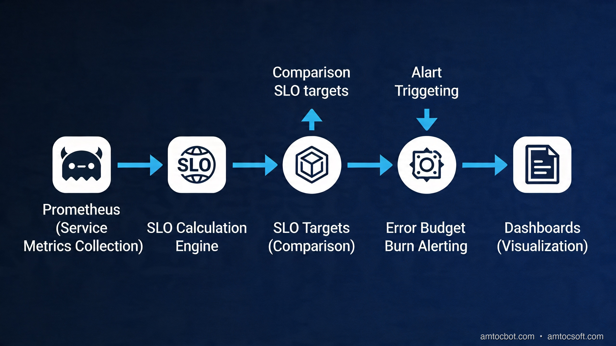
SLO Monitoring Pipeline

Implementation Guide: SLOs with Prometheus and Grafana

Step 1: Instrument Your Application

Start with request counters and latency histograms using the Prometheus client library for your language. Here's a complete example for a Go HTTP service:

package middleware

import (
    "net/http"
    "strconv"
    "time"

    "github.com/prometheus/client_golang/prometheus"
    "github.com/prometheus/client_golang/prometheus/promauto"
)

var (
    httpRequestsTotal = promauto.NewCounterVec(
        prometheus.CounterOpts{
            Name: "http_requests_total",
            Help: "Total number of HTTP requests by status class and endpoint",
        },
        []string{"method", "route", "status_class"},
    )

    httpRequestDuration = promauto.NewHistogramVec(
        prometheus.HistogramOpts{
            Name:    "http_request_duration_seconds",
            Help:    "HTTP request latency distribution",
            Buckets: []float64{0.005, 0.01, 0.025, 0.05, 0.1, 0.25, 0.5, 1, 2.5, 5, 10},
        },
        []string{"method", "route"},
    )
)

// SLOMiddleware wraps handlers to emit SLO-relevant metrics
func SLOMiddleware(route string, next http.HandlerFunc) http.HandlerFunc {
    return func(w http.ResponseWriter, r *http.Request) {
        start := time.Now()
        rw := &responseWriter{ResponseWriter: w, statusCode: http.StatusOK}

        next.ServeHTTP(rw, r)

        duration := time.Since(start).Seconds()
        statusClass := strconv.Itoa(rw.statusCode/100) + "xx"

        httpRequestsTotal.WithLabelValues(r.Method, route, statusClass).Inc()
        httpRequestDuration.WithLabelValues(r.Method, route).Observe(duration)
    }
}

type responseWriter struct {
    http.ResponseWriter
    statusCode int
}

func (rw *responseWriter) WriteHeader(code int) {
    rw.statusCode = code
    rw.ResponseWriter.WriteHeader(code)
}

Step 2: Define Recording Rules

Raw Prometheus metrics need pre-computation for SLO evaluation. Recording rules materialize expensive aggregations into new time series, making dashboard queries fast and alert evaluation reliable:

# prometheus/rules/slo-recording-rules.yaml
groups:
  - name: slo_recording_rules
    interval: 30s
    rules:

      # === Availability SLI: ratio of successful requests ===

      # 5-minute availability (for short-window burn rate)
      - record: job:http_request_success:rate5m
        expr: |
          sum(rate(http_requests_total{status_class!="5xx"}[5m])) by (job)
          /
          sum(rate(http_requests_total[5m])) by (job)

      # 30-minute availability
      - record: job:http_request_success:rate30m
        expr: |
          sum(rate(http_requests_total{status_class!="5xx"}[30m])) by (job)
          /
          sum(rate(http_requests_total[30m])) by (job)

      # 1-hour availability
      - record: job:http_request_success:rate1h
        expr: |
          sum(rate(http_requests_total{status_class!="5xx"}[1h])) by (job)
          /
          sum(rate(http_requests_total[1h])) by (job)

      # 6-hour availability (for slow-burn detection)
      - record: job:http_request_success:rate6h
        expr: |
          sum(rate(http_requests_total{status_class!="5xx"}[6h])) by (job)
          /
          sum(rate(http_requests_total[6h])) by (job)

      # === Latency SLI: ratio of requests under 500ms threshold ===

      - record: job:http_request_latency_ok:rate5m
        expr: |
          sum(rate(http_request_duration_seconds_bucket{le="0.5"}[5m])) by (job)
          /
          sum(rate(http_request_duration_seconds_count[5m])) by (job)

      - record: job:http_request_latency_ok:rate30m
        expr: |
          sum(rate(http_request_duration_seconds_bucket{le="0.5"}[30m])) by (job)
          /
          sum(rate(http_request_duration_seconds_count[30m])) by (job)

      # === Error Budget Burn Rate ===
      # SLO target = 99.5% → allowed error rate = 0.005
      # Burn rate = (1 - SLI) / (1 - SLO)

      - record: job:http_slo_burn_rate:5m
        expr: |
          (1 - job:http_request_success:rate5m) / (1 - 0.995)

      - record: job:http_slo_burn_rate:30m
        expr: |
          (1 - job:http_request_success:rate30m) / (1 - 0.995)

      - record: job:http_slo_burn_rate:1h
        expr: |
          (1 - job:http_request_success:rate1h) / (1 - 0.995)

      - record: job:http_slo_burn_rate:6h
        expr: |
          (1 - job:http_request_success:rate6h) / (1 - 0.995)

Step 3: Multi-Window Multi-Burn-Rate Alerting

This is the most important concept in production SLO alerting. Google's SRE workbook defines a four-tier alerting strategy using two time windows at each tier:

Tier Short Window Long Window Burn Rate Pages? Budget Consumed in...
Critical 5m 1h 14.4x Yes (P1) ~2 hours
High 30m 6h 6x Yes (P2) ~5 hours
Medium 2h 24h 3x Ticket ~10 hours
Low 6h 72h 1x Tracking 30 days (baseline)

The two-window requirement prevents false positives (short spikes trigger the short window but not the long window, so no alert fires) while ensuring responsiveness to sustained burns.

# prometheus/rules/slo-alerts.yaml
groups:
  - name: slo_burn_rate_alerts
    rules:

      # CRITICAL: Fast burn — page immediately
      # Both 5m AND 1h windows must exceed 14.4x burn rate
      - alert: SLOFastBurn
        expr: |
          job:http_slo_burn_rate:5m > 14.4
          and
          job:http_slo_burn_rate:1h > 14.4
        for: 2m
        labels:
          severity: critical
          team: platform
        annotations:
          summary: "CRITICAL: SLO fast burn on {{ $labels.job }}"
          description: |
            Service {{ $labels.job }} is burning error budget at {{ $value | printf "%.1f" }}x 
            the sustainable rate. At this rate, the 30-day budget will be exhausted in 
            approximately {{ (720 / $value) | printf "%.0f" }} hours.
            Current error rate: see Grafana SLO dashboard.
          runbook_url: "https://wiki.amtocsoft.com/runbooks/slo-fast-burn"

      # HIGH: Moderate fast burn — page with lower urgency
      - alert: SLOModerateHighBurn
        expr: |
          job:http_slo_burn_rate:30m > 6
          and
          job:http_slo_burn_rate:6h > 6
        for: 15m
        labels:
          severity: warning
          team: platform
        annotations:
          summary: "WARNING: SLO elevated burn on {{ $labels.job }}"
          description: |
            Service {{ $labels.job }} burn rate is {{ $value | printf "%.1f" }}x sustainable.
            30-day budget exhaustion in approximately {{ (120 / $value) | printf "%.0f" }} hours.
          runbook_url: "https://wiki.amtocsoft.com/runbooks/slo-elevated-burn"

      # MEDIUM: Slow burn — create ticket, no page
      - alert: SLOSlowBurn
        expr: |
          job:http_slo_burn_rate:2h > 3
          and
          job:http_slo_burn_rate:24h > 3
        for: 1h
        labels:
          severity: info
          team: platform
          action: ticket
        annotations:
          summary: "INFO: SLO slow burn on {{ $labels.job }}"
          description: |
            Service {{ $labels.job }} burn rate {{ $value | printf "%.1f" }}x — 
            budget will exhaust in approximately 10 days at this rate.
            Review recent deploys, error trends, and infrastructure changes.

Step 4: Grafana Dashboard Configuration

The Grafana dashboard should expose four key panels for each service:

  1. SLI Trend — the raw availability/latency ratio over the SLO window
  2. Error Budget Remaining — percentage of budget left in the current window
  3. Burn Rate — current multi-window burn rate as a gauge
  4. Request Volume — total request rate to contextualize error counts

Here's the core PromQL for the Error Budget Remaining panel:

# Error budget remaining as a percentage (30-day window)
# SLO = 99.5%, so total budget = 0.5% of requests

(
  1 - (
    (
      sum(increase(http_requests_total{status_class="5xx", job="$service"}[30d]))
    )
    /
    (
      sum(increase(http_requests_total{job="$service"}[30d]))
      * (1 - 0.995)
    )
  )
) * 100

Set thresholds: green above 50%, yellow 10-50%, red below 10%. This gives engineers an at-a-glance signal they can act on without reading the burn rate math themselves.


Comparison and Tradeoffs

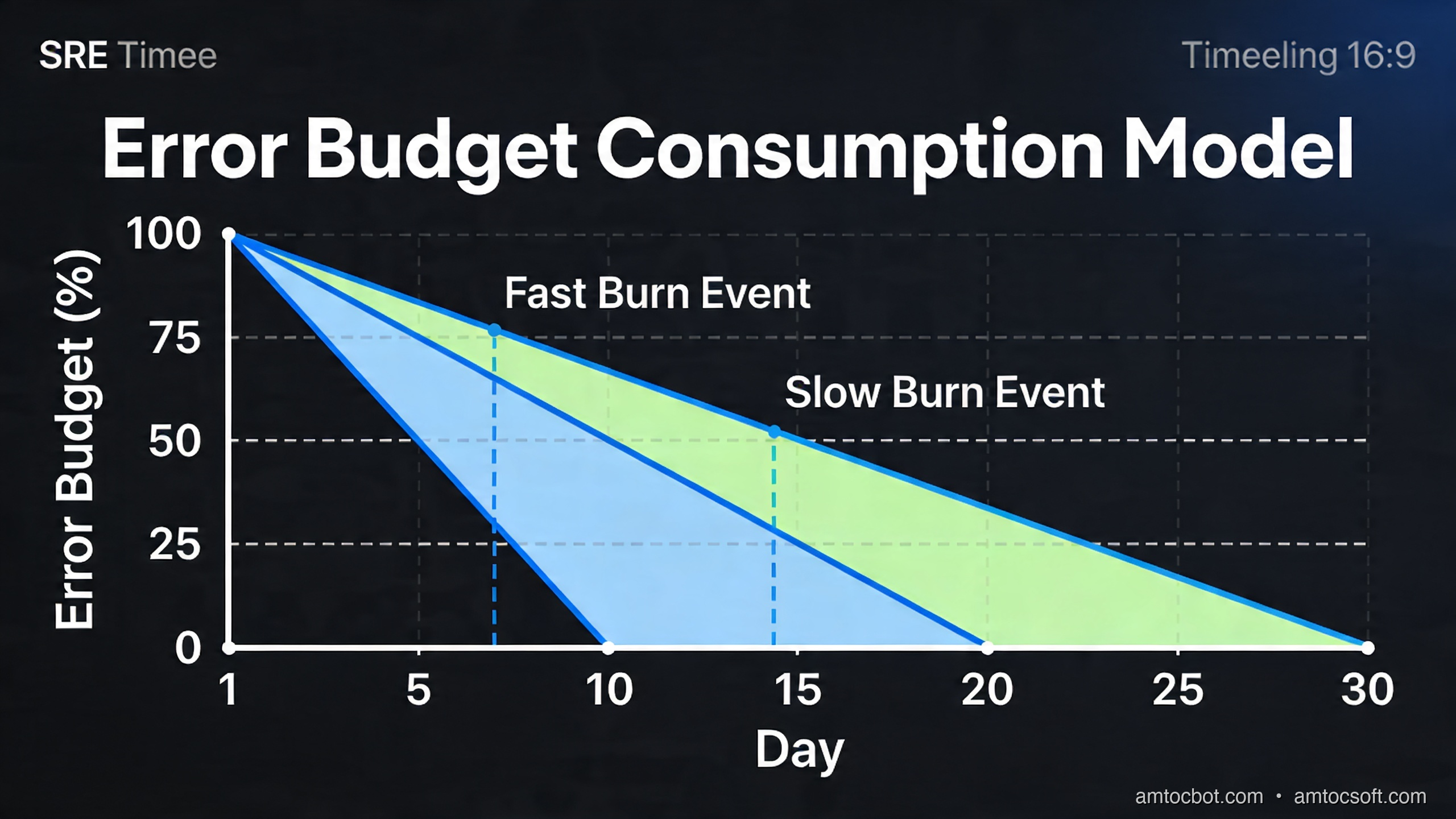
Error Budget Consumption Model

SLO Approaches: Pros, Cons, and When to Use Each

Approach Best For Limitations
Request-based SLOs HTTP APIs, gRPC services Requires instrumented request counters
Time-based SLOs Infrastructure health, batch jobs Less granular, misses partial failures
Composite SLOs Complex multi-service flows Harder to implement, more maintenance
Synthetic SLOs External-facing availability testing Doesn't capture backend degradation
Latency SLOs Latency-sensitive user flows Need histogram buckets at SLO thresholds

Request-based SLOs are the right default for most backend services. They measure what users actually experience (success or failure of individual interactions), they aggregate naturally over time windows, and they map cleanly onto the burn rate model.

Time-based SLOs work better for batch systems and infrastructure components where "requests" aren't meaningful. A database backup job either completes successfully in its window or it doesn't — that's better modeled as "minutes of successful operation" than as request success rate.

Composite SLOs attempt to capture end-to-end user journeys across multiple services. They're powerful for complex e-commerce or financial workflows where upstream service availability doesn't tell the full story, but they require careful dependency modeling and are significantly harder to maintain.

SLO Window Length Tradeoffs

Window Advantages Disadvantages
7-day rolling Reacts faster to trends More alert noise, budget recovered quickly
28/30-day rolling Standard, maps to billing cycles Slow to respond to slow burns
Quarter Strategic reliability view Too slow for operational response
Calendar month Maps to business reporting Budget "resets" create perverse incentives

Most teams use 30-day rolling windows for operational SLOs and quarterly aggregates for business reporting. Avoid calendar months — the "it resets on the 1st" dynamic encourages teams to exhaust their budget in the last week of the month.

SRE vs. Traditional Ops vs. DevOps

Dimension Traditional Ops DevOps SRE
Reliability target Maximize uptime Shared responsibility Error budget
Dev velocity Constrained by ops Teams own their stack Budget-gated
Failure response Blame assignment Post-deploy runbooks Blameless postmortem
Toil management Ad-hoc Some automation Explicit 50% cap
Alerting model Threshold-based Threshold-based Burn rate / SLO-based
Relationship model Dev vs Ops Shared but informal Embedded SREs, SLO contracts

Production Considerations

Chaos Engineering as SLO Validation

In 2026, chaos engineering has moved from Netflix-scale curiosity to mainstream practice. Tools like Chaos Mesh, Litmus, and AWS Fault Injection Simulator make it straightforward to inject failures in production (or production-like staging) and validate that your SLO monitoring detects them correctly.

A chaos experiment workflow integrated with SLOs looks like this:

#!/bin/bash
# chaos-experiment.sh — validate SLO alerting responds to injected failures

EXPERIMENT_NAME="latency-injection-api-gateway"
TARGET_SERVICE="api-gateway"
CHAOS_DURATION="300"  # 5 minutes

echo "[chaos] Starting experiment: $EXPERIMENT_NAME"
echo "[chaos] Recording baseline error budget..."

BASELINE_BUDGET=$(curl -s "http://prometheus:9090/api/v1/query" \
  --data-urlencode 'query=job:http_slo_error_budget_remaining:30d{job="api-gateway"}' \
  | jq -r '.data.result[0].value[1]')

echo "[chaos] Baseline budget remaining: ${BASELINE_BUDGET}%"

# Inject 200ms latency using Chaos Mesh
cat <<EOF | kubectl apply -f -
apiVersion: chaos-mesh.org/v1alpha1
kind: NetworkChaos
metadata:
  name: ${EXPERIMENT_NAME}
  namespace: default
spec:
  action: delay
  mode: all
  selector:
    namespaces: [default]
    labelSelectors:
      "app": "${TARGET_SERVICE}"
  delay:
    latency: "200ms"
    jitter: "50ms"
  duration: "${CHAOS_DURATION}s"
EOF

echo "[chaos] Latency injection active — monitoring for burn rate alert..."

# Wait and check if alert fired
sleep 360
ALERTS=$(curl -s "http://alertmanager:9093/api/v2/alerts" \
  | jq '[.[] | select(.labels.alertname == "SLOModerateHighBurn")]')

echo "[chaos] Alerts fired during experiment:"
echo "$ALERTS" | jq '.[].annotations.summary'

# Clean up
kubectl delete networkchaos ${EXPERIMENT_NAME}
echo "[chaos] Experiment complete. Check Grafana for budget impact."

Run chaos experiments at least quarterly, targeting different failure modes: latency injection, error injection, dependency outages, resource exhaustion. Document results in your runbooks — this is how you build confidence that your SLO monitoring will actually catch real incidents.

Toil Measurement and Reduction

SRE teams track toil explicitly. A simple toil ledger captures the recurring work that scales with service growth:

## Toil Inventory — Q2 2026

| Task | Frequency | Time/occurrence | Monthly hours | Automatable? |
|------|-----------|-----------------|---------------|--------------|
| Manual deployment approval for non-prod | Daily | 15min | 5h | Yes — auto-approve staging |
| Certificate rotation reminders | Monthly | 2h | 2h | Yes — cert-manager |
| Log archive cleanup | Weekly | 30min | 2h | Yes — lifecycle policy |
| Capacity scaling review | Weekly | 1h | 4h | Partial — HPA covers 80% |
| On-call handoff documentation | Weekly | 45min | 3h | Partial — auto-generated report |
| Manual SLO report for stakeholders | Monthly | 3h | 3h | Yes — Grafana reporting |

Total tracked toil: ~19h/month out of ~80h engineering = 24% (within 50% cap)
Priority automation targets: cert-manager, log lifecycle policy, Grafana reporting

Automation that eliminates toil directly improves reliability by reducing human error in repetitive operations. Every hour of toil eliminated is an hour recovered for reliability engineering that compounds over time.

Blameless Postmortem Structure

The postmortem is the most culturally significant artifact in SRE. A well-executed postmortem converts an incident into organizational learning. A poorly executed one (with blame) teaches engineers to hide problems. Here's the template structure that works:

# Postmortem: [Incident Title]

**Date**: YYYY-MM-DD
**Duration**: HH:MM — HH:MM UTC (X hours Y minutes)
**Severity**: P1 / P2 / P3
**Error Budget Impact**: X% of monthly budget consumed
**Author(s)**: [Names]
**Status**: Draft / In Review / Final

## Summary
One paragraph. What happened, what the user impact was, and what resolved it.
Written for an executive audience — no jargon.

## Timeline (UTC)
| Time | Event |
|------|-------|
| HH:MM | Anomaly first detectable in metrics |
| HH:MM | SLO burn rate alert fired |
| HH:MM | On-call acknowledged |
| HH:MM | Impact confirmed, incident declared |
| HH:MM | Root cause identified |
| HH:MM | Mitigation applied |
| HH:MM | Service fully recovered |
| HH:MM | Incident closed |

## Root Cause Analysis
What was the technical cause? Describe the contributing factors:
- Immediate cause (what triggered the failure)
- Contributing factors (what made it possible)
- Detection gaps (what slowed discovery)
- Response gaps (what slowed recovery)

Do NOT name individuals. Focus on systems, processes, and tooling.

## Impact Assessment
- User-visible impact: describe what users experienced
- Affected services: list impacted services and dependencies
- Error budget consumed: X of Y requests failed (Z% of monthly budget)

## What Went Well
- List things the team did right during the incident
- Include tooling, processes, and individual decisions

## What Could Be Improved
- Systemic gaps revealed by this incident
- Process breakdowns or missing automation

## Action Items
| Item | Owner | Due | Priority |
|------|-------|-----|----------|
| Add retry logic to dependent service calls | Platform team | 2026-05-01 | High |
| Add circuit breaker to payment service | Payments team | 2026-05-15 | High |
| Tune SLO alert thresholds for this failure mode | SRE | 2026-04-30 | Medium |

Track action items in your issue tracker with due dates. Review completion in the next monthly SRE review. Postmortems that generate action items that go nowhere are worse than no postmortem — they teach engineers that the process is theater.

Scaling SLO Monitoring: The Full Stack

flowchart TD A([Application Services]) -->|Prometheus metrics endpoint /metrics| B[Prometheus Scraper] A2([Synthetic Probes\nBlackbox Exporter]) --> B A3([Infrastructure Metrics\nNode Exporter, kube-state-metrics]) --> B B --> C[Recording Rules Engine\nPre-compute SLI/burn rates] C --> D[(Prometheus TSDB\nLong-term storage)] D --> E{Thanos / Mimir\nFederated storage layer} E --> F[Alertmanager\nRouting + Deduplication] E --> G[Grafana Dashboards\nSLO + Burn Rate views] F --> H[PagerDuty / OpsGenie\nOn-call routing] F --> I[Slack Alerts\nTeam channels] G --> J[Stakeholder Reports\nWeekly PDF exports] H --> K[Incident Commander\nOn-call engineer] K --> L[Runbooks\nAutomated remediation] L --> M([Resolved Incident]) M --> N[Postmortem\nAction items → backlog] N --> A

In 2026, the reference stack for production SLO monitoring is:

  • Instrumentation: OpenTelemetry SDK (language-native) exporting to Prometheus format
  • Collection: Prometheus with recording rules for SLI/burn rate pre-computation
  • Long-term storage: Thanos or Grafana Mimir for multi-month retention (required for 30-day SLOs)
  • Alerting: Alertmanager with multi-window burn rate rules → PagerDuty/OpsGenie for P1/P2
  • Dashboards: Grafana with Pyrra or Sloth for SLO dashboard generation
  • Chaos testing: Chaos Mesh (Kubernetes) or AWS FIS for regular validation

Pyrra and Sloth deserve a special mention. These tools take SLO definitions as CRDs (Custom Resource Definitions) and automatically generate the Prometheus recording rules, alerting rules, and Grafana dashboards:

# pyrra/slo-api-gateway.yaml
apiVersion: pyrra.dev/v1alpha1
kind: ServiceLevelObjective
metadata:
  name: api-gateway-availability
  namespace: monitoring
spec:
  description: "API Gateway HTTP availability SLO"
  target: "99.5"
  window: 30d
  serviceMonitorSelector:
    matchLabels:
      app: api-gateway
  indicator:
    ratio:
      errors:
        metric: http_requests_total{job="api-gateway",status_class="5xx"}
      total:
        metric: http_requests_total{job="api-gateway"}

Pyrra reads this definition and generates all the recording rules, burn rate alerts, and a pre-built Grafana dashboard. For teams managing dozens of services, this is the difference between SLO practice being sustainable or becoming a maintenance burden.


Conclusion

SRE is not a role — it's a practice, a set of principles, and a cultural shift in how engineering organizations think about reliability. The core insight that unlocked it all: reliability has a cost, unreliability has a cost, and the right amount of each depends on your users, your business, and your engineering velocity.

SLIs give you a precise, user-focused measure of reliability. SLOs give your team a shared target and the operational tools to make good decisions. Error budgets convert that target into a currency that aligns development velocity with reliability investment. Burn rate alerting gives you early warning before users notice. Blameless postmortems convert failures into learning. Toil reduction converts manual work into engineering capacity.

For developers making the transition to reliability thinking, the practical starting point is simple: instrument your service, define one SLI, set one SLO, and build a burn rate alert. You don't need the full Pyrra stack on day one. You need one dashboard that tells you whether your service is burning budget faster than it can recover, and one alert that wakes someone up when it is.

From that foundation, every piece of this guide builds naturally. Run a chaos experiment to validate your alerting. Write your first postmortem. Track your first toil item and automate it away. Expand to latency SLOs. Add composite SLOs for critical user journeys. Adopt Pyrra or Sloth to scale SLO management across dozens of services.

The teams that do this well don't just have more reliable services — they ship faster, have fewer midnight incidents, and spend their engineering time on work that matters. That's the real promise of SRE in 2026.


Sources

About the Author

Toc Am

Founder of AmtocSoft. Writing practical deep-dives on AI engineering, cloud architecture, and developer tooling. Previously built backend systems at scale. Reviews every post published under this byline.

LinkedIn X / Twitter

Published: 2026-04-15 · Written with AI assistance, reviewed by Toc Am.

Get These In Your Inbox

Weekly deep-dives on AI engineering, no fluff. Join the newsletter →

Subscribe (free)

Or grab the book ($39, ~100 pages) · Buy me a coffee

Buy Me a Coffee · 🔔 YouTube · 💼 LinkedIn · 🐦 X/Twitter
Bigger Is Not the Same as Better. The Job That Moved Is the Phone, Not the Lab.

Bigger is a plan. The phone is the receipt. The brief for this cycle is a question: does bigger always mean better in AI? The 2026 answer i...