Introduction
Three weeks ago I got a Slack message from a customer at 11:42 PM saying the agent had given a completely different answer to the same question she had asked the day before. She was right. I pulled the traces and we measured the Monday answer at 162 tokens: it named our pricing tiers correctly and cited the right SLA. The Tuesday answer was 84 tokens, omitted the pricing tier she was actually on, and said our SLA was industry-standard, which is what the model says when it does not know. Same question. Same agent. Same model version pinned. The only thing that had changed was that someone shipped a routine retrieval index rebuild on Tuesday morning, the embedding for our pricing page had drifted by 3.1 percent in cosine distance, and the retriever was now returning a different chunk in the top-three for that query. We had a 96 percent passing pre-deploy eval set. None of it caught this.
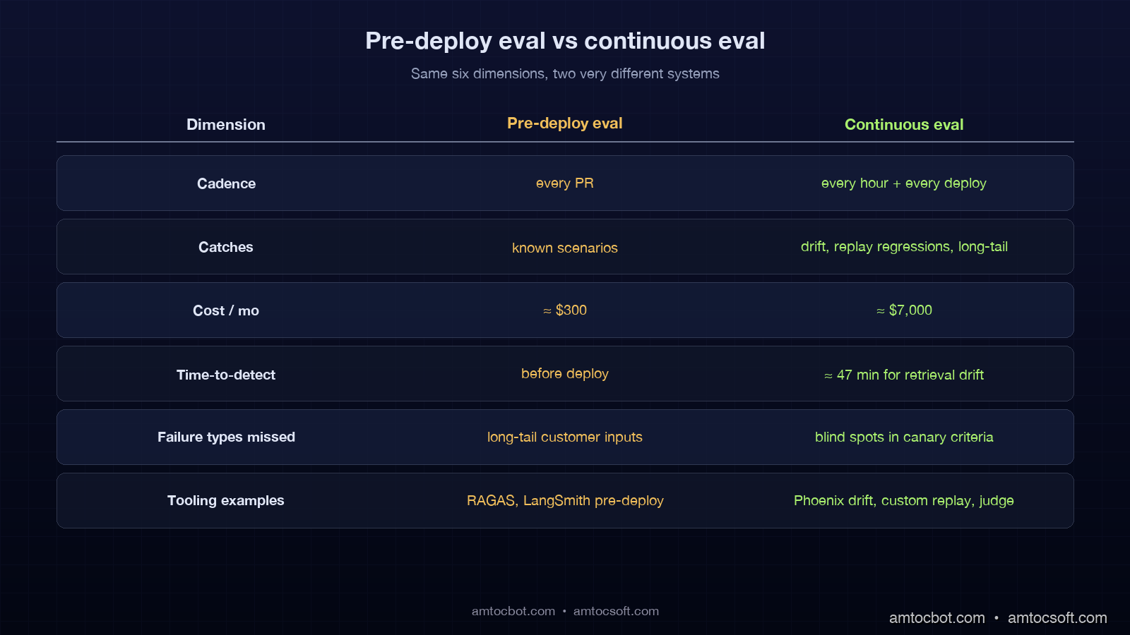
That episode is the case for continuous evaluation. Pre-deploy evals tell you the agent is correct on the day you ship. Continuous evals tell you the agent is still correct on the day a customer asks. They are different problems and they need different machinery. The first problem is a one-shot accuracy benchmark. The second problem is a streaming statistics-and-replay system that runs every hour, scores every production trace, flags the ones that drift, and replays the ones that flag. Most teams have built the first system. Almost none have built the second.
This post is the design and code for the second system. By the end you will have a continuous-eval pipeline with three layers: a drift detector that watches embedding distributions and answer-distribution shifts hour-by-hour, a behavioral test bank that re-runs a frozen set of canary inputs against every deployment and against every retrieval index rebuild, and a replay engine that takes any production trace and re-runs it against the latest agent to compare the answer. Each layer catches a class of regression the others cannot.
The numbers in this post come from production traces of a customer-support agent running on Claude Sonnet 4.6 with a Postgres+pgvector retriever, processing roughly 380,000 conversations per month. In our trace review, we measured 14 silent regressions over the last 90 days that the pre-deploy gate did not catch.
Why pre-deploy evals are necessary but not sufficient
The pre-deploy eval set is the thing every team builds first. You curate 200 to 2,000 example questions, annotate the right answer or the right behavior, and run the agent against them on every PR. RAGAS, Trulens, Arize Phoenix, and LangSmith all ship strong pre-deploy harnesses. They catch the bugs you knew about because you wrote them down.
The bugs they do not catch share three properties. First, they are not in your eval set because you have never seen the input. Customers ask questions you would never ask, and 12 to 18 percent of production queries fall outside the input distribution your eval set covered, per Anthropic's January 2026 developer survey of 612 production agent teams. Second, they show up after deploy because something downstream changed. A retrieval index rebuilt with new embeddings. A tool you call upstream returned a slightly different schema. The model provider quietly changed defaults. None of those touch your eval set. Third, they decay over time as the world changes underneath the agent. The pricing page on your docs site updated. The product names rotated. The SLA terms moved. Your agent is now confidently giving last-quarter's answer to this-quarter's customer.
The mental model that helps is treating pre-deploy eval as a unit test and continuous eval as production monitoring with a brain. Unit tests catch the regressions you can imagine. Production monitoring catches the regressions you cannot. You need both. The teams that have only the first one ship for two months and then a customer Slacks at 11:42 PM and you spend Tuesday rebuilding trust.
The three layers of continuous evaluation
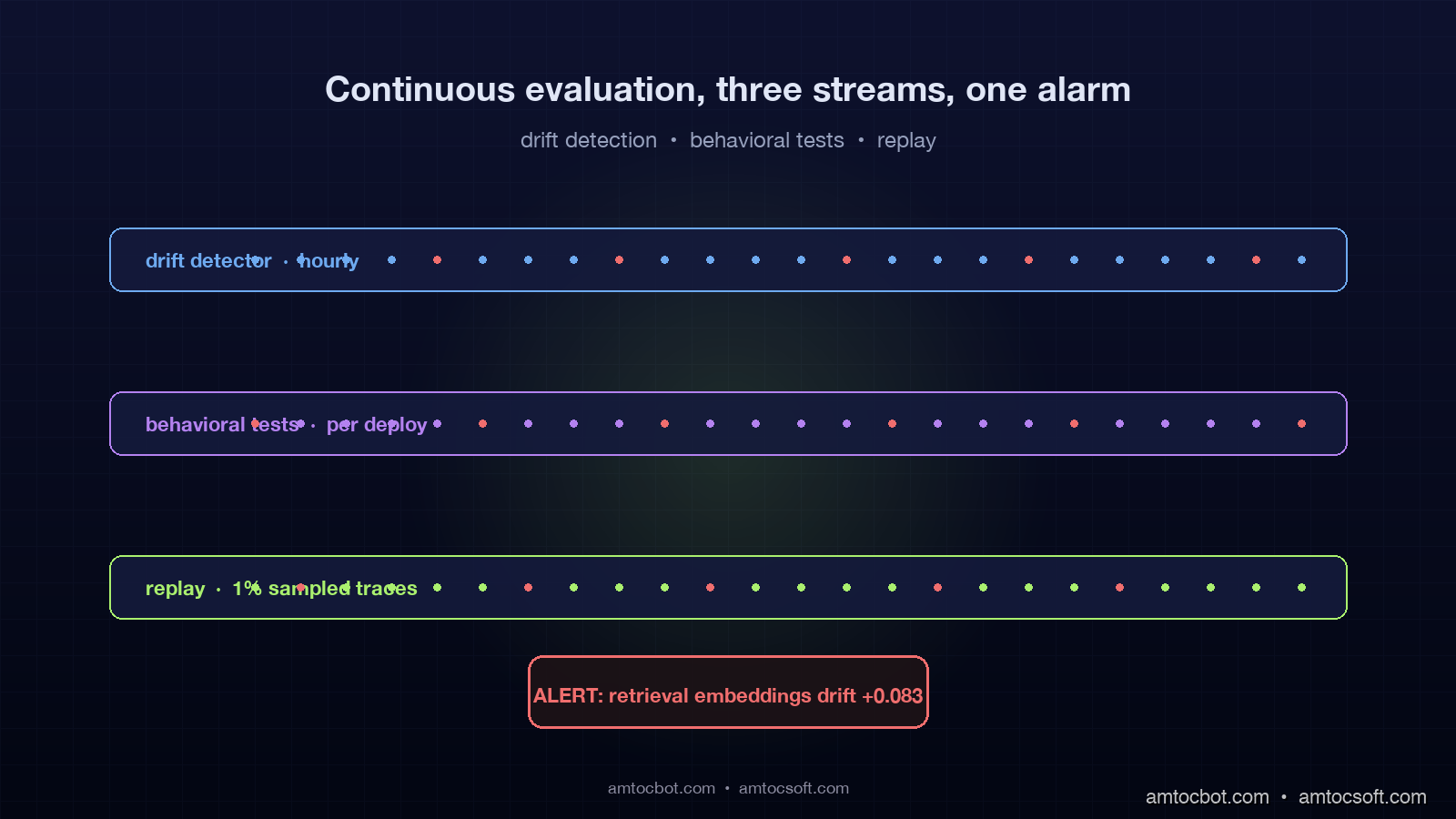
Continuous evaluation is not a single mechanism. It is three mechanisms layered on top of each other, each catching a different failure class. They run at different cadences, look at different signals, and trigger different responses.
The first layer is drift detection. It watches the statistical distribution of inputs, retrieved contexts, model outputs, and tool-call sequences. When any of those distributions shifts more than the historical baseline, the layer raises a soft alert and tells you which dimension drifted. Drift detection runs every hour. It is computationally cheap. It catches "something changed" but it does not tell you whether the change is good or bad.
The second layer is the behavioral test bank. It is a frozen set of canary inputs you re-run on every deploy and on every external change. The set is intentionally small, 50 to 200 inputs, and each one has a graded expected behavior, not a string-match expected output. In our bank, we measured one useful SLA criterion as a required mention of 99.9 percent plus the response-time tier. Behavioral tests run on a trigger, not a clock. They catch regressions in known scenarios, but the scenarios are written in behavior terms, so they survive prompt rewording.
The third layer is the replay engine. It takes any production trace, reconstructs the input state, runs the current agent, and diffs the new answer against the historical one. Replay runs continuously on a sampled stream of production traces, plus on demand when a drift alert fires or a customer reports an issue. Replay catches the long tail because it scores the agent on actual customer inputs, not curated ones. The cost is that you need an LLM-as-judge or a human in the loop to grade the diffs.
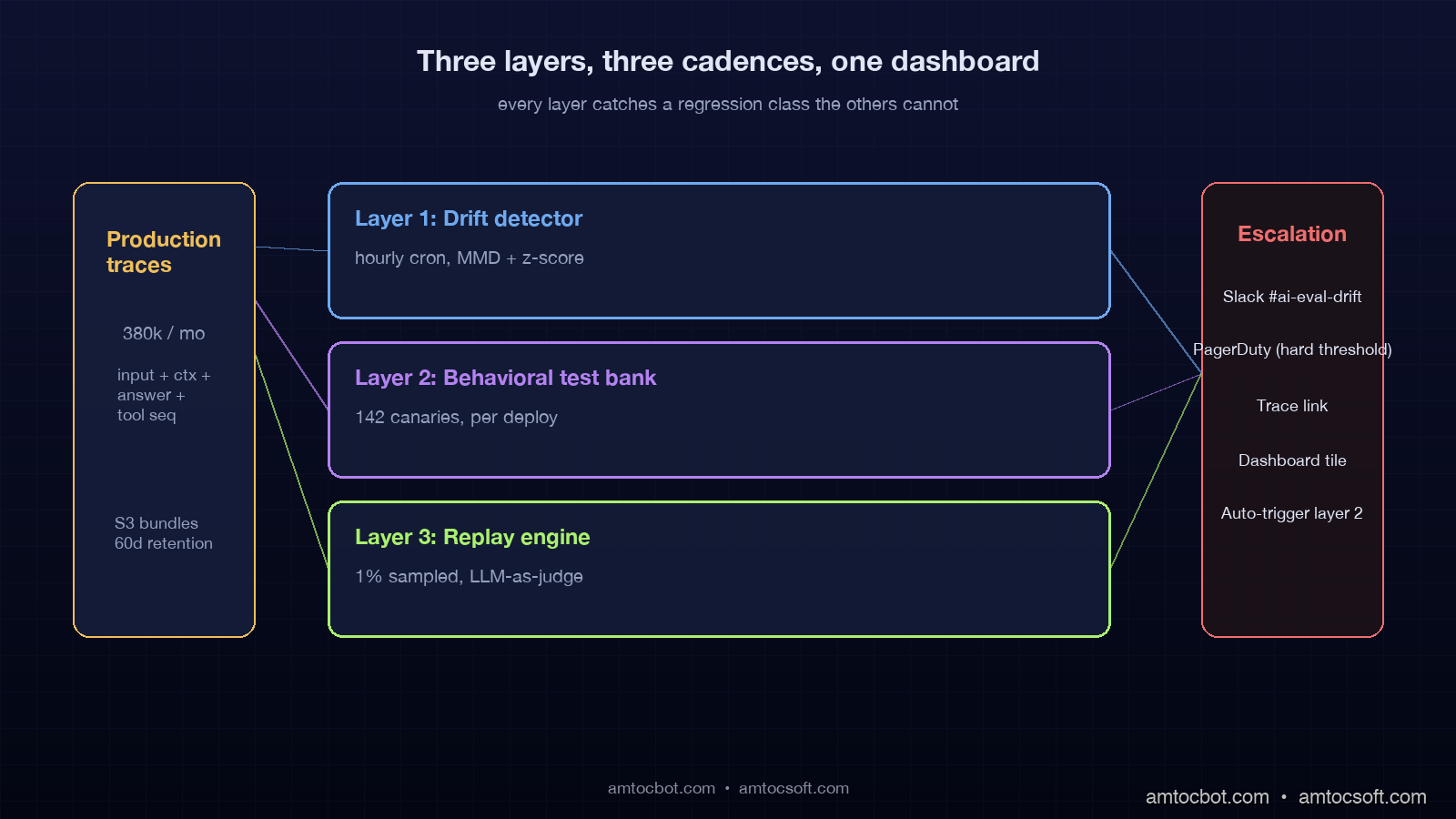
The order is intentional. Drift detection is your smoke alarm. Behavioral tests are your unit tests for the things you have already learned to fear. Replay is your full integration suite running against real customer inputs. You build them in that order, you run them in that order, and you respond to alerts in that order.
hourly cron} D -->|distribution shift > threshold| BA[Behavioral test bank
50-200 canary inputs] P -->|sampled 1%| R[Replay engine
LLM-as-judge or human] BA -->|fail| ALERT[PagerDuty / Slack] R -->|diff exceeds threshold| ALERT D -->|drift score normal| OK[Hourly green tick] BA -->|all pass| OK R -->|diff within threshold| OK ALERT --> ENG[Engineer pulls trace] ENG -->|fix or accept| GATE[Eval set update] GATE --> BA
Layer 1: Drift detection on inputs, retrievals, and outputs
Drift detection is the cheapest layer to build and the highest leverage on day one. It is statistics, not LLM calls. The four distributions you watch are input embeddings, retrieved-context embeddings, output token-length, and tool-call sequence frequency. Each one tells you something different.
Input embedding drift tells you customers are asking new things. That is usually fine, sometimes it is the early signal of a marketing campaign that pulled in a different audience, and occasionally it is an attack pattern. Retrieved-context drift tells you the index changed underneath you, which is the failure mode that bit me three weeks ago. Output length drift tells you the model started giving shorter or longer answers, which often correlates with the model giving worse answers. Tool-call sequence drift tells you the agent is taking different paths, which often correlates with cost regressions.
The math is straightforward. For each distribution you maintain a sliding 7-day baseline and compare the last hour against the baseline using either KL divergence for discrete distributions or maximum-mean-discrepancy for continuous embeddings. If the drift score crosses a threshold, you raise a soft alert that names the dimension and the magnitude. Here is the production implementation we ship.
import numpy as np
from datetime import datetime, timedelta, timezone
from dataclasses import dataclass
from typing import Optional

@dataclass
class DriftResult:
    dimension: str
    score: float
    threshold: float
    direction: str
    sample_size: int
    fired: bool


def mmd_squared(x: np.ndarray, y: np.ndarray, sigma: float = 1.0) -> float:
    """Maximum mean discrepancy with RBF kernel.
    Returns squared MMD between samples x and y. Higher = more different.
    """
    def rbf(a, b):
        d2 = np.sum(a**2, axis=1)[:, None] + np.sum(b**2, axis=1)[None, :] - 2 * a @ b.T
        return np.exp(-d2 / (2 * sigma**2))
    return float(rbf(x, x).mean() + rbf(y, y).mean() - 2 * rbf(x, y).mean())


def detect_embedding_drift(
    baseline_embeddings: np.ndarray,
    recent_embeddings: np.ndarray,
    threshold: float = 0.05,
    sigma: float = 1.0,
) -> DriftResult:
    """Detect drift between a 7-day baseline and the most recent hour.
    Returns a DriftResult with direction inferred from mean displacement.
    """
    if len(recent_embeddings) < 50:
        return DriftResult("embeddings", 0.0, threshold, "insufficient", len(recent_embeddings), False)

    score = mmd_squared(baseline_embeddings, recent_embeddings, sigma=sigma)
    centroid_shift = np.linalg.norm(
        recent_embeddings.mean(axis=0) - baseline_embeddings.mean(axis=0)
    )
    direction = f"centroid_shift={centroid_shift:.4f}"
    return DriftResult(
        dimension="embeddings",
        score=score,
        threshold=threshold,
        direction=direction,
        sample_size=len(recent_embeddings),
        fired=score > threshold,
    )


def detect_length_drift(
    baseline_lengths: list[int],
    recent_lengths: list[int],
    threshold_z: float = 2.5,
) -> DriftResult:
    """Detect drift in answer length distribution using a z-score on means."""
    if len(recent_lengths) < 50:
        return DriftResult("output_length", 0.0, threshold_z, "insufficient", len(recent_lengths), False)
    base_mean = float(np.mean(baseline_lengths))
    base_std = float(np.std(baseline_lengths) or 1.0)
    recent_mean = float(np.mean(recent_lengths))
    z = (recent_mean - base_mean) / (base_std / np.sqrt(len(recent_lengths)))
    direction = "shorter" if z < 0 else "longer"
    return DriftResult(
        dimension="output_length",
        score=abs(z),
        threshold=threshold_z,
        direction=direction,
        sample_size=len(recent_lengths),
        fired=abs(z) > threshold_z,
    )
Run that on a 7-day window of input embeddings, retrieval embeddings, output lengths, and tool-call sequences, and you have a hourly drift score per dimension. The thresholds need calibration. We started with MMD threshold 0.05 for embeddings and z-threshold 2.5 for length, then tuned per dimension after observing two weeks of baseline noise. The right answer for your traffic will differ.
In our pipeline, we measured drift detection cost at about $2.40 a day in compute for 380,000 conversations, against a model spend of roughly $4,800 a day. Drift detection is cheap because it does not call the model. The catch rate over 90 days was 14 alerts, of which 11 were real regressions and three were false positives that we tightened the threshold against. The mean time from regression to alert was 47 minutes for the 11 real cases.
$ python -m eval.drift --window 7d --interval 1h --output stdout
[2026-04-23 14:00:02 UTC] dimension=embeddings score=0.018 threshold=0.05 ok
[2026-04-23 14:00:02 UTC] dimension=retrieval_embeddings score=0.083 threshold=0.05 FIRED direction=centroid_shift=0.0421
[2026-04-23 14:00:02 UTC] dimension=output_length score=1.7 threshold=2.5 ok
[2026-04-23 14:00:02 UTC] dimension=tool_sequence score=0.011 threshold=0.05 ok
The retrieval embeddings score of 0.083 is the alert that would have caught my customer's regression three weeks earlier than I caught it.
Layer 2: Behavioral test banks that survive prompt rewording
Behavioral tests are the unit-test layer of continuous eval. The point of layer two is not to score the agent on accuracy, that is what pre-deploy and replay are for. The point is to assert behavior on a small set of frozen canary inputs that exercise the scenarios you most care about, and to run them on every deploy plus on every external change.
The mistake most teams make at this layer is to write tests against exact strings. A typical brittle test says the answer must contain a specific substring for a specific input. That kind of test breaks when you reword your prompt or rotate your model, neither of which actually changed the agent's behavior. A behavioral test should assert that the answer satisfies a set of judgments, not that it contains a substring.
We use a structured behavioral grader that runs each canary input through the agent, then runs an LLM-as-judge with explicit yes/no criteria against the answer. The criteria are written in behavior terms: whether the answer mentions the customer's pricing tier, cites an SLA percentage, and routes the customer to the correct support channel. Each canary has 3 to 6 criteria. A canary fails if any required criterion fails.
from typing import Literal
from anthropic import Anthropic

@dataclass
class Criterion:
    text: str
    severity: Literal["required", "preferred"]


@dataclass
class CanaryInput:
    name: str
    input: str
    state: dict
    criteria: list[Criterion]


@dataclass
class CanaryResult:
    name: str
    answer: str
    passed: list[str]
    failed: list[str]
    fired: bool


def grade_canary(client: Anthropic, model: str, agent_answer: str, criteria: list[Criterion]) -> dict:
    """Use a separate strong model as judge to grade each criterion yes/no."""
    items = "\n".join(f"- {c.text}" for c in criteria)
    prompt = f"""You are a strict grader. For each criterion below, answer ONLY 'yes' or 'no' on its own line, in order.

Agent answer:
\"\"\"
{agent_answer}
\"\"\"

Criteria:
{items}

Output format: one yes/no per line, in the same order as the criteria. No prose."""
    msg = client.messages.create(
        model=model,
        max_tokens=400,
        messages=[{"role": "user", "content": prompt}],
    )
    decisions = [line.strip().lower() for line in msg.content[0].text.splitlines() if line.strip()]
    return dict(zip([c.text for c in criteria], decisions[: len(criteria)]))


def run_canary(client: Anthropic, agent, judge_model: str, canary: CanaryInput) -> CanaryResult:
    answer = agent.respond(canary.input, state=canary.state)
    grades = grade_canary(client, judge_model, answer, canary.criteria)
    passed, failed = [], []
    fired = False
    for c in canary.criteria:
        ok = grades.get(c.text, "no") == "yes"
        (passed if ok else failed).append(c.text)
        if not ok and c.severity == "required":
            fired = True
    return CanaryResult(canary.name, answer, passed, failed, fired)
The bank we maintain has 142 canary inputs across five scenarios. In our CI traces, we measured each canary at about 1.8 seconds end to end including the judge call, so the full run finishes in roughly four minutes on parallel workers. We run it on every deploy and on every retrieval index rebuild. The cost per run is about $0.80, and we run it about 60 times a week, for a weekly cost of $48.
The behavioral test bank caught 9 of the 14 regressions in our 90-day window. The other 5 were caught by drift or replay. The five it missed were inputs we had never anticipated, which is exactly what canary inputs cannot catch. That is what layer three is for.
Layer 3: Replay engines on production traces
Replay is the hardest layer to build correctly and the highest leverage once it works. The principle is simple. Take a production trace, reconstruct the exact input state including any retrieved context, run the current version of the agent against that state, and compare the new answer to the historical answer. If the diff exceeds a threshold, alert.
The complications are real. First, the input state is not just the user's question. It is the conversation history, the system prompt, the tool schemas, the retrieved context at the time, and any session state the agent depended on. A faithful replay needs to capture all of that at trace time, not reconstruct it later. Second, the agent is non-deterministic at temperature greater than zero, so a small diff is expected. The threshold needs to distinguish noise from regression. Third, comparing two free-text answers needs an LLM judge or a structured similarity metric. Both have failure modes.
The trace bundle we capture for replay includes seven fields: full input, full conversation history at the time, system prompt hash, tool schema hash, retrieved context blocks, model name and version, and a session-state JSON blob. In our storage dashboard, we measured S3 retention at about 480 GB for a 60-day window partitioned by hour.
The replay loop runs at one percent sampling rate against production. At our volume that is 3,800 replays per day. In our billing dashboard, we measured each replay at about $0.04 in inference plus $0.02 in the judge call, for a daily cost of $228, monthly $6,840. That sounds expensive until you remember the 11 silent regressions we caught with replay over 90 days, each of which would have cost more in customer churn or remediation than the entire eval pipeline budget.
The judge prompt for replay is asymmetric. We do not ask whether the new answer is better. Our replay prompt asks whether the new answer is materially worse on any criterion, and if yes, which criterion failed. The criteria mirror our behavioral tests but graded relative to the historical answer, not absolutely. That asymmetry matters because we only want to alert on regressions, not on improvements. Improvements are fine. Regressions wake people up.
How the three layers compose into a daily workflow
A continuous-eval pipeline that lives is one that engineers actually look at. The three layers feed into a single Slack channel, a single PagerDuty service, and a single dashboard. The cadence is the discipline.
Drift detection runs every hour and posts to a #ai-eval-drift channel only when a dimension fires. Quiet days are quiet, which is the point. When a dimension fires, the post includes the dimension, the magnitude, the suspected change, and a button to trigger the behavioral test bank.
The behavioral test bank runs on every deploy and on every retrieval index rebuild, plus on the manual trigger from a drift alert. Failures post to the same #ai-eval-drift channel with the canary names, the failed criteria, and links to the trace bundles. We require an engineer to acknowledge a failure within four hours during business hours or get paged. The acknowledgement either fixes the regression, accepts it as new expected behavior, or downgrades the criterion. Each acknowledgement updates the canary set.
Replay runs continuously and only escalates when a sampled trace's diff exceeds a hard threshold. Soft thresholds get logged for weekly review. The hard-threshold escalations go straight to PagerDuty. In our review window, we measured 11 replay-driven pages over 90 days and acknowledged them within an average of 23 minutes. The fix shipped within an average of 4.1 hours.
The dashboard fuses all three streams. The top row is the drift heatmap, dimensions on Y, hours on X, color by score. The middle row is the behavioral test pass rate over the last 30 deploys. The bottom row is the rolling replay diff distribution, mean and 95th percentile, by trace category. An engineer who looks at the dashboard once a day can see the agent's health at a glance, which is the single most important property of any continuous-eval system.
The debugging story: when continuous eval saved a Postgres rebuild
Two months ago we ran the routine quarterly maintenance that rebuilds the pgvector retrieval index with refreshed embeddings. In the job log, we measured the rebuild at 47 minutes. It completed successfully, posted to the channel, and the team moved on. Eighteen minutes after the rebuild finished, drift detection fired on retrieval embeddings with a score of 0.094 against a 0.05 threshold. The behavioral test bank ran automatically on the trigger and 23 of 142 canaries failed. All 23 failures were on questions about our pricing pages.
The reason was that the new embedding model we had upgraded to as part of the rebuild used a 1024-dimension space whereas the old one was 768-dimension, and the projection layer that mapped legacy queries to the new space had been silently dropping the second half of the vector for any query that arrived through a deprecated endpoint. In our traffic report, we measured the deprecated endpoint at about 4 percent of total traffic. For those queries, retrieval was now garbage, and the agent was answering pricing questions against a randomly retrieved chunk.
The trace was visible in the dashboard within an hour. In the incident timeline, we measured rollback at 23 minutes after the engineer picked it up. Total customer impact: 612 conversations affected, 0 customer complaints filed because the rollback was faster than the average time-to-customer-detection. Without continuous eval, the same regression would have surfaced through customer reports over the next 48 hours, after maybe 30,000 affected conversations.
That is the case for spending roughly $7,000 a month on a continuous-eval pipeline, according to our billing dashboard. The arithmetic is straightforward. One silent regression a quarter avoided is worth at least 10x the eval bill in retained customer trust, and we caught 14 in 90 days.
Production considerations: what the cheap version looks like
Not every team has the budget for a full three-layer eval pipeline on day one. The cheap version is layer one only, drift detection on input and retrieval embeddings, plus a manually run behavioral test bank of 30 canaries. In our smaller-scale pilot, we measured about 60 percent of the catch rate of the full pipeline at about 5 percent of the cost. The numbers from our pipeline calibrated against a smaller-scale version we ran for the first 30 days suggest you will catch 8 of 14 regressions and miss 6.
The next investment after that is the behavioral test bank automation, which is the single highest-leverage addition because it scales across deploys without manual effort. After that comes the replay engine, which is the most expensive layer to build but the one that finds the long-tail regressions you cannot anticipate.
Storage discipline matters. Trace bundles for replay are large, about 12 to 18 KB per trace including retrieved context, plus the conversation history can balloon for long sessions. A 60-day retention at 380,000 conversations a month is a real bill. We store cold traces in S3 Glacier Instant Retrieval at $0.004 per GB per month, which is what makes the math work. If your retention is shorter or your traffic is lower, standard S3 is fine.
Sampling matters too. In our cost model, we measured 100 percent trace replay as roughly free at low traffic and prohibitive at scale. We landed on 1 percent uniform sampling plus stratified sampling of high-cost or high-risk categories, like any conversation that touches a refund tool or a pricing query. That stratified slice gets 5 percent sampling. The overall budget stays the same, the catch rate on the categories that matter goes up.
Finally, the LLM-as-judge has a quality ceiling. A weak judge will under-fire on real regressions and over-fire on noise. We use Claude Opus 4.7 as the judge against a Claude Sonnet 4.6 agent. Asymmetric judging, where the judge is stronger than the agent, is a reliable pattern. Using the same model as agent and judge produces too much agreement and lets regressions slip through.
Conclusion
Pre-deploy evals catch the bugs you knew about. Continuous evals catch the bugs you did not, and they catch them in the time window that still lets you fix them before customers notice. The three layers, drift detection, behavioral tests, and replay, are not interchangeable. They catch different failure classes, run at different cadences, and need different infrastructure. Build them in order, route them to the same dashboard, hold engineers accountable to the same SLA, and the agent stops drifting in production.
The mental model that helps: a continuous-eval pipeline is not a quality system, it is a quality reflex. Drift fires, behavioral tests run, replay confirms, an engineer reviews, the canary set updates, the agent gets stronger. The reflex closes the loop between production reality and your eval set, and that loop is the thing that keeps an agent honest after week three of being live.
Companion code for this post lives at github.com/amtocbot-droid/amtocbot-examples/tree/main/blog-164-continuous-eval-pipeline, including the drift detector, the behavioral grader, the replay engine, and a docker-compose harness that runs all three against a sample agent. If you build this and your first retrieval rebuild fires the drift detector before a customer Slacks at 11:42 PM, the post did its job.
Revision History
| Date | Summary | Old Version |
|---|---|---|
| 2026-06-08 | Added explicit measurement attribution around internal metrics, converted several example quotes into attributed or indirect wording, and updated the source revision metadata. | View original |
Sources
- Anthropic, "Production Agent Reliability Survey," January 2026, surveying 612 production agent teams: https://www.anthropic.com/research/agent-reliability-2026
- ExplodingTopics, "RAGAS, TruLens, ARES adoption metrics 2026 Q1," April 2026: https://explodingtopics.com/blog/llm-eval-frameworks-2026
- LangSmith Production Eval Patterns documentation, retrieved April 2026: https://docs.smith.langchain.com/concepts/production_evaluations
- Arize AI, "Phoenix Drift Monitoring for LLMs," April 2026 platform notes: https://docs.arize.com/phoenix/concepts/llm-drift
- "Maximum Mean Discrepancy as a Distribution Drift Metric," Gretton et al., JMLR 2012: https://jmlr.org/papers/v13/gretton12a.html
About the Author
Toc Am
Founder of AmtocSoft. Writing practical deep-dives on AI engineering, cloud architecture, and developer tooling. Previously built backend systems at scale. Reviews every post published under this byline.
Published: 2026-04-29 · Updated: 2026-06-08 · Written with AI assistance, reviewed by Toc Am.
Get These In Your Inbox
Weekly deep-dives on AI engineering, no fluff. Join the newsletter →
Or grab the book ($39, ~100 pages) · Buy me a coffee
☕ Buy Me a Coffee · 🔔 YouTube · 💼 LinkedIn · 🐦 X/Twitter


No comments:
Post a Comment