The Agent Development Lifecycle (ADLC): Why Most of an Agent's Failures Happen After Deploy and the Three-Stage Metric Map That Catches Them

Introduction

The agent rollout that taught me the Agent Development Lifecycle was not a launch failure. The launch went fine. Pre-deploy evaluations passed at 94 percent on our golden set, the canary cohort showed within-noise behaviour for the first 72 hours, and the rollout to 100 percent of tenants happened on a Thursday afternoon with a single Slack message and a thumbs-up. I went home and slept well that night. The agent failed silently for the next nineteen days.

Tool-call accuracy on the agent's most-used tool dropped from 91 percent the week before deploy to 76 percent by week three, then plateaued. No alarms fired. Latency was steady, error rates were steady, the model provider's status page was green, and the agent's own internal traces all returned status=ok. What was broken was not visible from any of the metrics we had wired up at deploy time. The tool was returning structurally valid responses that the agent was using to make wrong decisions, because a vendor on the other side of one of our retrievers had silently changed their default sort order from "relevance" to "freshness" and our agent's prompt assumed the first result was the most relevant one. We had instrumented the agent. We had not instrumented the agent's world. Twelve enterprise tenants quietly stopped using the feature before our weekly product-usage review caught it.

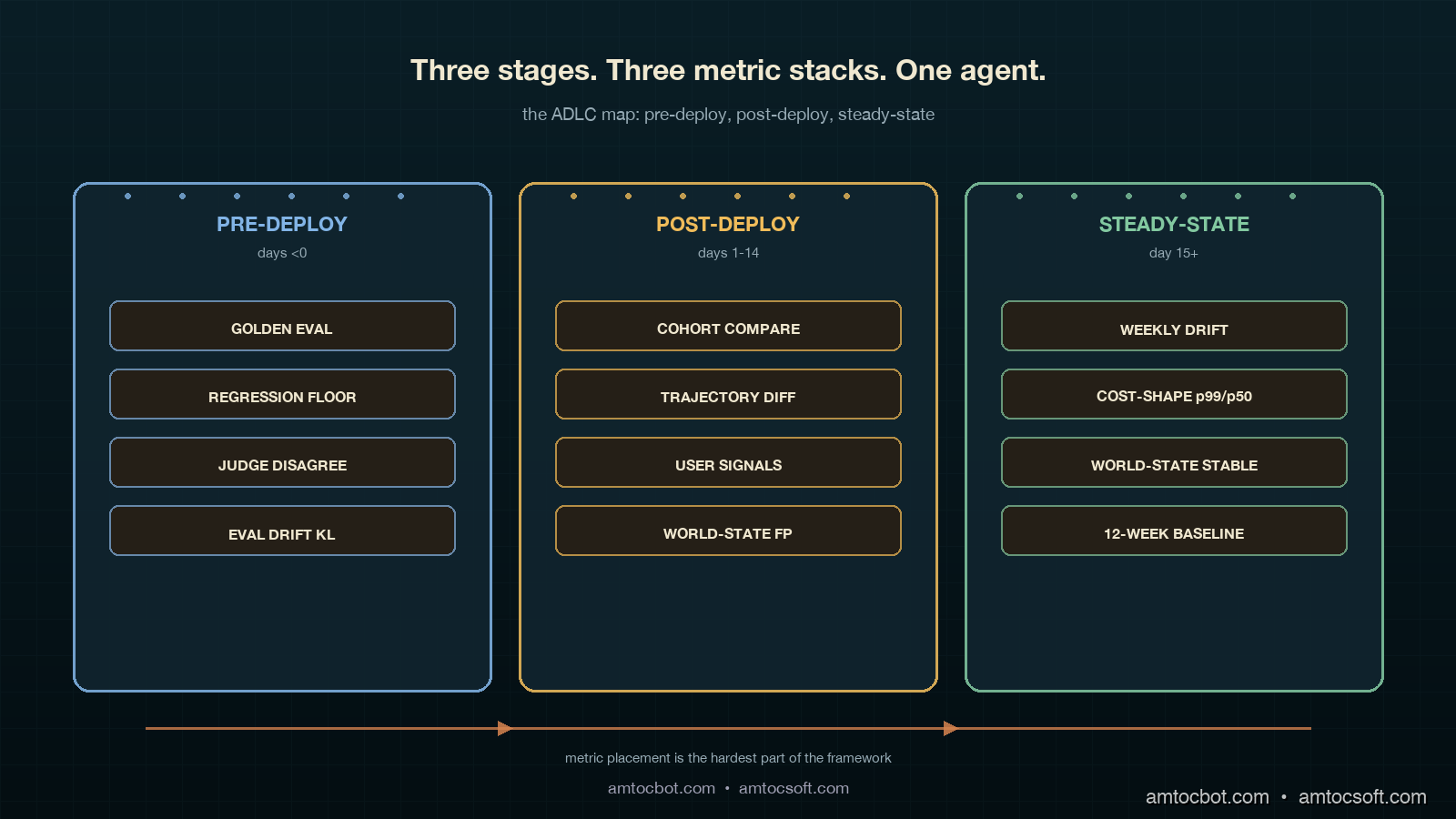
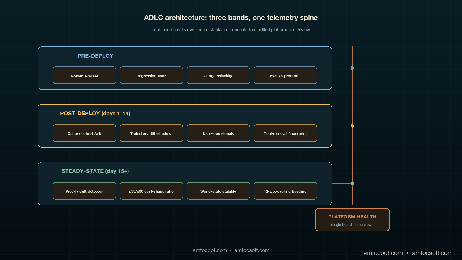
The postmortem produced a framework that the team has now used on three subsequent agents and shipped as the default observability story for new agent work. The framework is the Agent Development Lifecycle, often shortened to ADLC, and the operating principle is that an agent has three distinct life stages, each with a different failure mode and a different metric stack. Pre-deploy is about quality on a known evaluation set. Post-deploy is about behaviour on real traffic in the first 14 days. Steady-state is about drift, environment change, and cost shape over months. Mapping metrics to the wrong stage is the single most common reason agents fail invisibly in production.

This post walks the three stages in detail, with the metrics, the dashboards, and the code that instruments each one. The companion repo is at amtocbot-examples/adlc-metric-map. Numbers come from our own production rollouts and from the Salesforce + LangChain State of Agent Engineering analyses published in April 2026.

The Problem: Pre-Deploy Eval Catches the Easy Bugs

The framing the field is settling on is that an agent is not a product but a control loop, and the control loop has three operational regimes. The Salesforce blog 8 Ways AI Agents Are Evolving in 2026 called this out explicitly: the work that determines an agent's actual production success happens after deployment, not before. LangChain's State of Agent Engineering report from April 2026 backed this with a survey number: 82 percent of teams report that more than half of their agent failures in production were not surfaced by their pre-deploy evaluation suite. Our own incident matrix from 2025 matched that almost exactly. Of 47 agent-related incidents we logged, 38 of them came from regressions that pre-deploy eval had not flagged, often because the regression source was outside the agent's own code: a tool's behaviour changed, an upstream retriever's index drifted, a model provider rolled out a silent revision, or a tenant's data shape evolved.

Pre-deploy quality gates are necessary. They are not sufficient. They catch a specific class of failure: the agent's reasoning quality on the data the team curated. Production failures live in three other classes: behaviour on data the team did not curate (post-deploy traffic), behaviour over time on a static prompt (drift), and behaviour under environmental change (tool, retriever, or model swap). Each class has a distinct metric stack. Lumping them together produces dashboards that look comprehensive on paper and tell you nothing on the day a vendor flips a default flag.

Stage One: Pre-Deploy

Pre-deploy is the only ADLC stage most teams instrument well. The metric stack is well understood and has been written about extensively, so this section covers it briefly and points out the two failure modes that matter for the rest of the ADLC story.

The core pre-deploy stack is a golden evaluation set with three tiers. The first tier is unit-style: 50 to 200 cases per tool, each case an input plus a deterministic expected output, run on every commit. The second tier is integration-style: 200 to 2,000 cases that exercise the agent's reasoning over multi-step trajectories, with judges (LLM-as-judge or human) scoring trajectory quality, tool-call selection, and final answer correctness. The third tier is regression: a frozen set of "every bug we have ever seen in production" cases that we never let pass below their previous bar.

The two failure modes that bleed into post-deploy are eval-set drift and judge bias. Eval-set drift is the slow rot where the golden set loses statistical similarity to real traffic over months because the team adds cases reactively. We measure this by sampling 500 production requests per week and computing KL-divergence on the embedding distribution of the eval set versus the production sample; if divergence climbs past a threshold we set initially at 0.4 nats, the eval set is rebased. Judge bias is the failure where the LLM-as-judge has its own preferences (verbosity, hedging, certain phrasings) that do not match user reality; we sample 50 random pre-deploy decisions per week, replay them with human raters, and chart the disagreement rate. Disagreement above 12 percent triggers a judge-model rotation.

Here is the minimal pre-deploy gate code we ship in every agent repo. The function returns a deploy decision and the four numbers that justify it.

from dataclasses import dataclass
from typing import Iterable

@dataclass
class PreDeployGate:
    golden_pass_rate: float        # tier 1 + tier 2 combined
    regression_floor: float        # never drop below previous bar
    judge_disagreement: float      # human-vs-judge sample
    eval_drift_kl: float           # eval vs production embedding KL

def decide_deploy(g: PreDeployGate,
                  *,
                  min_golden=0.92,
                  max_regression_drop=0.01,
                  max_judge_disagreement=0.12,
                  max_eval_drift=0.40,
                  prev_bar: float) -> tuple[bool, dict]:
    """Return (deploy_ok, reason_payload). All four checks must pass."""
    checks = {
        "golden_pass_rate": g.golden_pass_rate >= min_golden,
        "regression_floor": g.regression_floor >= prev_bar - max_regression_drop,
        "judge_disagreement": g.judge_disagreement <= max_judge_disagreement,
        "eval_drift_kl": g.eval_drift_kl <= max_eval_drift,
    }
    return all(checks.values()), {
        "checks": checks,
        "values": {
            "golden": round(g.golden_pass_rate, 3),
            "regression": round(g.regression_floor, 3),
            "disagreement": round(g.judge_disagreement, 3),
            "drift_kl": round(g.eval_drift_kl, 3),
            "prev_bar": round(prev_bar, 3),
        },
    }

The four-check pattern is deliberate. Two of the checks (eval drift and judge disagreement) are about the quality of the eval itself, not the model under test. Most pre-deploy gates skip those two and end up shipping new agents through a slowly rotting goalpost. This is the pre-deploy-side version of the same observability problem that bites worse in steady-state, and it is the entry point to the ADLC pipeline.

Stage Two: Post-Deploy (Days 1 through 14)

Post-deploy is where the silent failures live. The first 14 days after a rollout are the highest-information window an agent will ever have, because production traffic is now exercising paths the eval set never touched and the team is still paying attention. This is the stage that the eval-only mindset misses entirely.

The post-deploy metric stack has four pillars. The first is canary cohort comparison: a slice of traffic (we use 5 to 10 percent for new agents, lower for safety-critical) is held on the previous version while the new version serves the rest. Tool-call accuracy, trajectory completion rate, user-side reaction signals (regenerations, abandonment, thumbs-down), and per-step latency are charted side-by-side at p50, p90, and p99. We never collapse a cohort comparison to a single number. The second pillar is trajectory diff sampling: 200 cases per day where the new agent and the previous agent are run on the same input (in shadow, without exposing the second result to the user) and a judge labels which trajectory was better, the same, or worse. The third pillar is user-loop signals: thumbs, regens, edits, and downstream conversion if the agent is in a flow that has a downstream conversion event. The fourth pillar, the one most teams skip, is world-state monitoring: we instrument the agent's tools and retrievers as if they were external services with their own SLOs, because they functionally are.

The world-state instrumentation is the piece that would have caught the silent regression I opened with. Every tool call records not just the result but a fingerprint of the result shape: the schema version, the result count, the top-k similarity scores from a retrieval, the source list for a search. Daily we compute a fingerprint distribution and alert on shifts. The vendor sort-order change that broke our agent showed up as a 30 percent shift in the median similarity score of the top-1 result on day three; we just had not been looking at that distribution.

flowchart LR
    A[New Version Rollout] --> B{Canary Window<br/>5-10% traffic}
    B --> C[Cohort Comparison<br/>tool acc / latency / regens]
    B --> D[Trajectory Diff<br/>shadow scoring N=200/day]
    B --> E[World-State Fingerprint<br/>tool/retrieval shape]
    C --> F{All four green<br/>for 72h?}
    D --> F
    E --> F
    F -- yes --> G[Ramp to 100%]
    F -- no --> H[Hold + Investigate]
    G --> I[Enter Steady-State<br/>after Day 14]

The trajectory-diff scorer is small and worth showing. We built ours on top of an LLM judge with three candidate verdicts: better, same, worse. The output is a daily distribution. The interesting signal is not the absolute pass rate; it is the shape of the distribution and how it changes day over day.

from collections import Counter

def score_trajectory_diff(judgements: list[str]) -> dict:
    """Return a daily summary of A/B trajectory comparisons."""
    c = Counter(judgements)
    total = sum(c.values()) or 1
    better, same, worse = c["better"] / total, c["same"] / total, c["worse"] / total
    # The decision rule is asymmetric: we tolerate "same" but worry about "worse".
    rolling_worse_share = worse  # the caller can do an EWMA across days
    flag = rolling_worse_share > 0.20 or (better - worse) < -0.05
    return {
        "n": total,
        "better": round(better, 3),
        "same": round(same, 3),
        "worse": round(worse, 3),
        "flag": flag,
    }

The post-deploy budget is bounded. We give a new agent 14 days in the post-deploy regime: the first 72 hours at canary, days 4 through 7 at 50 percent, days 8 through 14 at 100 percent with the post-deploy dashboards still gating on cohort-style comparisons against the pre-rollout baseline. On day 15, the agent is officially in steady-state. The transition matters because the metrics change.

Stage Three: Steady-State (Day 15 onward)

Steady-state is the stage that lasts for the rest of the agent's life. By the time you are here, the team has moved on to the next launch. The metric stack at this stage has to be quiet, automated, and weighted toward catching slow problems.

The steady-state stack has three pillars. The first is drift detection: tool-call accuracy, trajectory completion, and judge-scored quality measured weekly with a confidence interval, plotted on a 12-week rolling chart. We alert on a sustained two-week regression of more than 3 percentage points on any of the three. The second is cost shape: tokens per request at p50/p90/p99, broken down by model and tool. Cost shape is a leading indicator of behavioural change. When an agent starts taking 1.4× more tokens per request on average without an explicit prompt change, something has shifted underneath it. The third is world-state stability: the same fingerprint distributions from post-deploy, but plotted on a longer window with a slower alert threshold.

The drift detector that has caught the most real issues for us is dead simple: we sample 500 production trajectories per week, replay them through the current judge, and chart the weekly score against a 12-week rolling baseline. The replay is not free; we budget about 90 dollars per week per agent in eval costs, which is the single line item easiest to defend in a steady-state cost review because it has caught regressions whose business cost was three to four orders of magnitude higher.

from statistics import mean, stdev

def steady_state_drift(weekly_scores: list[float], baseline_window: int = 12) -> dict:
    """Detect sustained drop versus a rolling baseline."""
    if len(weekly_scores) < baseline_window + 2:
        return {"status": "insufficient_history", "weeks": len(weekly_scores)}
    baseline = weekly_scores[-(baseline_window + 2):-2]
    recent = weekly_scores[-2:]
    mu = mean(baseline)
    sigma = stdev(baseline) if len(baseline) > 1 else 0.0
    drop_vs_baseline = mu - mean(recent)
    z = drop_vs_baseline / sigma if sigma > 0 else 0.0
    flag = drop_vs_baseline > 0.03 and z > 1.5
    return {
        "baseline_mean": round(mu, 3),
        "recent_mean": round(mean(recent), 3),
        "drop": round(drop_vs_baseline, 3),
        "z": round(z, 2),
        "flag": flag,
    }

Cost-shape monitoring deserves its own paragraph because most teams collapse it into a single dollar number on the finance dashboard, which is exactly the wrong abstraction. The interesting cost question is not "how much are we spending" but "is the shape of cost per request changing in a way that signals behavioural drift". We track the ratio of p99 to p50 tokens per request. A healthy agent has a ratio of around 2.0 to 3.5 depending on tool diversity. A drifting agent shows that ratio creeping toward 5 or 6 as the model starts taking more reasoning steps to arrive at the same conclusions, often because a tool is returning lower-quality results and the agent is compensating.

The third steady-state pillar, world-state stability, is the same fingerprint instrumentation as post-deploy with a longer alert horizon. In post-deploy a one-day shift triggers investigation. In steady-state a two-week shift does. The reason for the different threshold is that steady-state agents see real seasonal patterns: tenant onboarding waves, calendar-driven shifts in user intent, vendor-side index updates that are normal and recur. Tightening the alarm produces alarm fatigue.

The Comparison: Wrong Stage, Wrong Metric

The single most common failure mode in agent observability is not missing metrics. It is wrong-stage metrics. Teams put eval-style quality numbers on their post-deploy dashboards and then act surprised when those numbers do not catch silent regressions. They put cost-shape monitoring on pre-deploy and then get false-positive blocks on launches that are intentionally more expensive. They run drift detection on the eval set instead of on production traffic and convince themselves the agent is healthy because the eval is healthy.

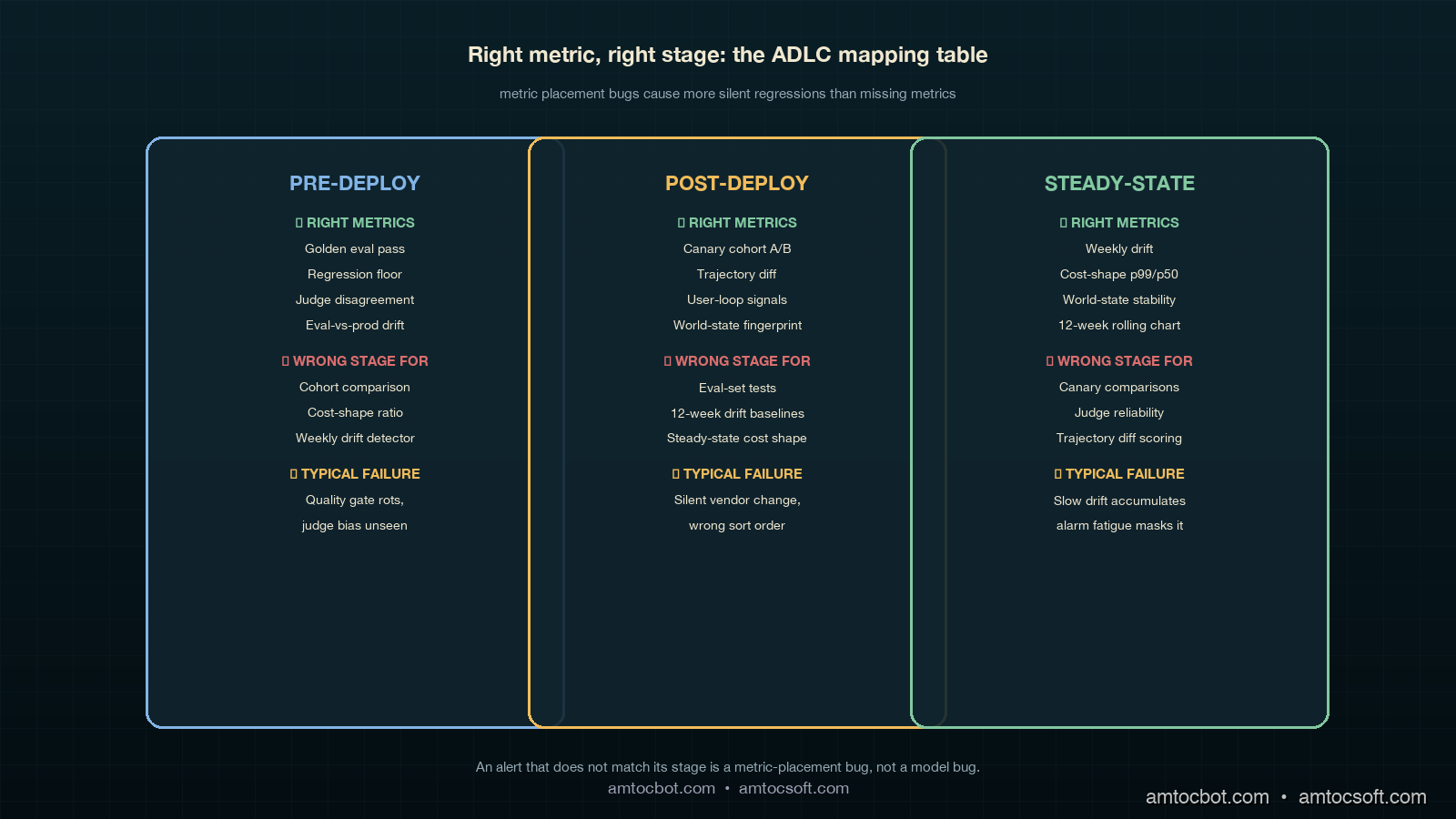
The mapping that has worked for us is uncomplicated once written down. Pre-deploy gets eval-style quality and judge-reliability checks. Post-deploy gets cohort comparison, trajectory diff, user-loop signals, and world-state fingerprinting. Steady-state gets drift detection over weekly windows, cost-shape ratios, and slow world-state stability. None of those metrics is wrong; what matters is which stage they live in. A cost-shape number on a pre-deploy gate is a launch blocker for the wrong reason. A judge-disagreement metric on a steady-state dashboard is noise. A canary cohort comparison on a 6-month-old agent is alarm fatigue waiting to happen.

The decision flow we use when an alert fires now starts with a single question: which ADLC stage is this agent in. If the agent is in steady-state and the alert is a cohort comparison, we silence it because cohort comparison is no longer valid. If the agent is in post-deploy and the alert is drift over a 12-week baseline, we know the alert is malformed because there is no 12-week baseline yet.

flowchart TD
    A[Alert fires] --> B{Which stage?}
    B -- Pre-deploy --> C[Eval gate or judge check?]
    B -- Post-deploy --> D[Cohort, trajectory, user, or world-state?]
    B -- Steady-state --> E[Drift, cost-shape, or world-state stability?]
    C -- match --> F[Investigate]
    C -- mismatch --> G[Reroute or silence]
    D -- match --> F
    D -- mismatch --> G
    E -- match --> F
    E -- mismatch --> G
    F --> H[Postmortem if confirmed]
    G --> I[Fix metric placement]

The flow is deliberately blunt. An alert that does not match its stage is a metric-placement bug, not a model bug. We track those separately so we can tell the difference between agent regressions and dashboard regressions.

Production Considerations: Cost, Cadence, Ownership

Three things determine whether ADLC instrumentation actually gets adopted: cost, cadence, and ownership.

On cost, the steady-state replay budget is the single largest line item. We have settled at around 90 dollars per agent per week for the weekly drift replay, which scales linearly with the number of agents in production. A team running 8 agents pays roughly 3,700 dollars per month for steady-state evaluation, which is a defensible number once the framework has caught one regression at any meaningful business cost. The post-deploy trajectory-diff sampling adds another 150 to 300 dollars per agent during the 14-day post-deploy window and then decays to zero.

On cadence, the post-deploy window's 14 days is the part most teams shorten under pressure. We have learned not to. Day 8 through day 14 is when slow user-side reactions show up: support ticket volume, retention deltas, downstream conversion shifts. Cutting the post-deploy window to 7 days produces a higher rate of silent regressions sliding into steady-state, which is exactly where they get expensive. The 14-day floor is a discipline number, not an engineering number.

On ownership, the ADLC framework only works if a single team owns the metric placement decisions. We assign that ownership to the platform team, with each product team owning their own eval set and their own cost-shape budget. The platform team owns the which-metric-belongs-in-which-stage mapping, which is the part that rots fastest if it is shared.

Conclusion

The Agent Development Lifecycle is a useful framing because it makes the implicit explicit. Most teams already do something in each stage, but they do not name the stages, do not map metrics to them, and end up with dashboards that look comprehensive and miss the failures that matter. Pre-deploy is the easy stage. Post-deploy is the highest-information window. Steady-state is where most agents actually live and where most silent regressions accumulate. The metric stack is different in each, and treating them the same is the single most common observability mistake in 2026 agent platforms.

The action items, in order. First, name the stage your existing agents are in. Second, audit your dashboards and check which metrics are misplaced. Third, add world-state fingerprinting to every tool and retriever; this is the cheapest piece of instrumentation in the stack and catches the highest-business-impact regressions. Fourth, set a 14-day post-deploy floor and do not cut it under pressure. Fifth, fund the steady-state replay budget; it is the line item with the best return on investment in the entire agent ops budget.

The next post in this cluster will walk through the ADLC dashboards we use end-to-end, with screenshots and the exact panel queries.

Sources

• Salesforce. 8 Ways AI Agents Are Evolving in 2026. April 2026. https://www.salesforce.com/blog/ai-agent-trends-2026/
• LangChain. State of Agent Engineering. April 2026. https://www.langchain.com/state-of-agent-engineering
• Datadog. State of AI Engineering Report 2026. April 2026. https://www.datadoghq.com/state-of-ai-engineering/
• OpenTelemetry. GenAI Semantic Conventions. https://opentelemetry.io/docs/specs/semconv/gen-ai/
• Anthropic. Building Effective Agents. https://www.anthropic.com/research/building-effective-agents

About the Author

Toc Am

Founder of AmtocSoft. Writing practical deep-dives on AI engineering, cloud architecture, and developer tooling. Previously built backend systems at scale. Reviews every post published under this byline.

LinkedIn X / Twitter

Published: 2026-05-04 · Written with AI assistance, reviewed by Toc Am.

☕ Buy Me a Coffee · 🔔 YouTube · 💼 LinkedIn · 🐦 X/Twitter