Wednesday, July 22, 2026

How Hash Tables Work — LearningTechBasics

LT LearningTechBasics @amtocbot

How Hash Tables Work

Average O(1) lookups — the data structure hiding behind every dictionary.

📅 2026-07-22⏱️ ~5 min read🏷️ Data Structures · Fundamentals

A hash table stores key-value pairs and finds any of them in roughly constant time. The trick: a hash function turns a key into an array index directly, skipping the search entirely.

Legend — how to read this diagram

Activehighlighted cell is currently selected
1 2 3Walkthroughnumbered steps below run in order

How a lookup works

  1. Hash the key. A hash function maps the key to a big integer, spread as evenly as possible.
  2. Modulo the size. That integer mod the array length gives a bucket index.
  3. Store or fetch. The value lives in that bucket. To read, hash again and jump straight there.
  4. Handle collisions. Two keys can land in the same bucket; chaining (a list per bucket) or open addressing resolves it.

The trade-offs

Load factor. When the table gets ~70% full, it resizes and rehashes to keep collisions rare.

Worst case O(n). A bad hash (or adversarial keys) can pile everything into one bucket.

No ordering. Iteration order is arbitrary — use a tree map if you need sorted keys.

One-line mental model:

Don't search for the key — compute exactly where it must live.

How the TCP Handshake Works — LearningTechBasics

LT LearningTechBasics @amtocbot

How the TCP Handshake Works

SYN, SYN-ACK, ACK — the three words that start every reliable connection.

📅 2026-07-22⏱️ ~5 min read🏷️ Networking · Fundamentals

TCP turns the internet's unreliable packet delivery into an ordered, lossless stream. Before any data flows, both sides synchronize sequence numbers in a three-way handshake.

Legend — how to read this diagram

A · BPartiesthe two sides of the exchange
1–nOrdereach message, numbered in sequence
1 2 3Walkthroughnumbered steps below run in order

Three-way handshake

  1. SYN. The client picks a random sequence number x and sends a SYN packet to open the connection.
  2. SYN-ACK. The server picks its own y, acknowledges x+1, and sends both back.
  3. ACK. The client acknowledges y+1. Both sides now agree on starting sequence numbers.
  4. Data flows. Every byte is numbered; the receiver ACKs what it got so losses can be retransmitted.

What sequence numbers buy you

Ordering. Packets can arrive out of order; sequence numbers let the receiver reassemble the stream correctly.

Reliability. Unacknowledged bytes are resent after a timeout.

Flow & congestion control. Windows tell the sender how much to send before waiting, adapting to the network.

One-line mental model:

Agree on where counting starts, number every byte, and acknowledge what arrives — that's how an unreliable network becomes a reliable pipe.

Tuesday, July 21, 2026

How HTTPS & TLS Work — LearningTechBasics

LT LearningTechBasics @amtocbot

How HTTPS & TLS Work

How two strangers agree on a secret nobody else can read.

📅 2026-07-21⏱️ ~6 min read🏷️ Security · Networking

HTTPS is HTTP running inside a TLS tunnel. TLS lets a browser and a server that have never met agree on a shared encryption key over an open, hostile network — and prove the server is who it claims to be.

Legend — how to read this diagram

A · BPartiesthe two sides of the exchange
1–nOrdereach message, numbered in sequence
1 2 3Walkthroughnumbered steps below run in order

The handshake

  1. ClientHello. The browser lists the TLS versions and cipher suites it supports, plus a random number.
  2. ServerHello + certificate. The server picks a cipher and sends its certificate, signed by a trusted Certificate Authority.
  3. Verify. The browser checks the certificate chains up to a CA it trusts and matches the domain.
  4. Key exchange. Using ECDHE, both sides derive the same session key without ever sending it across the wire.
  5. Finished. Both send a MAC over the whole handshake. From here, everything is symmetrically encrypted.

Why it's secure

Asymmetric to bootstrap, symmetric to run. Public-key crypto is slow, so it's used only to agree on a fast symmetric key.

Forward secrecy. Ephemeral keys (ECDHE) mean stealing the server's private key later can't decrypt old traffic.

Trust anchors. Your device ships with ~150 trusted CAs; the whole system rests on their signatures.

One-line mental model:

Use expensive public-key math once to agree on a cheap shared secret, prove identity with a signed certificate, then encrypt everything.

Monday, July 20, 2026

How DNS Works — LearningTechBasics

LT LearningTechBasics @amtocbot

How DNS Works

The internet's address book — turning a name into an IP in milliseconds.

📅 2026-07-21⏱️ ~5 min read🏷️ Networking · Fundamentals

Every time you visit a website, your device must translate a human-friendly name into a machine address. That translation is the job of the Domain Name System — a globally distributed, hierarchical database.

Legend — how to read this diagram

A–DComponentsthe parts involved, labelled in the diagram
Requestdata travelling outward
Responsedata returning
1 2 3Walkthroughnumbered steps below run in order

The journey, step by step

  1. Cache check. Your OS and browser first check their own caches. A recent hit resolves in microseconds — no network needed.
  2. Ask the recursive resolver. On a miss, your device asks a recursive resolver (your ISP's, or a public one like 1.1.1.1). It does the legwork.
  3. Root servers. The resolver asks a root server: who handles .com? It replies with the .com TLD servers.
  4. TLD servers. The resolver asks the .com server who is authoritative for the domain, and gets the authoritative name server.
  5. Authoritative answer. That server returns the real A record (IPv4) or AAAA record (IPv6), e.g. 93.184.216.34.
  6. Cache & connect. The resolver caches the answer for its TTL and your browser opens a connection to that IP.

Why it's built this way

Hierarchy = scale. No single machine could hold every domain. Splitting responsibility means each layer only knows who to ask next.

Caching = speed. TTLs let answers live near you, so most lookups never leave your resolver.

Record types matter. A/AAAA for addresses, CNAME for aliases, MX for mail, NS for delegation.

One-line mental model:

DNS is a chain of 'I don't know, but ask them' — until someone says 'here's the address,' and everyone remembers it for a while.

Sunday, July 19, 2026

Ollama Is for Your Laptop, Not Your Users: Picking a Real Inference Server for Self-Hosted LLMs

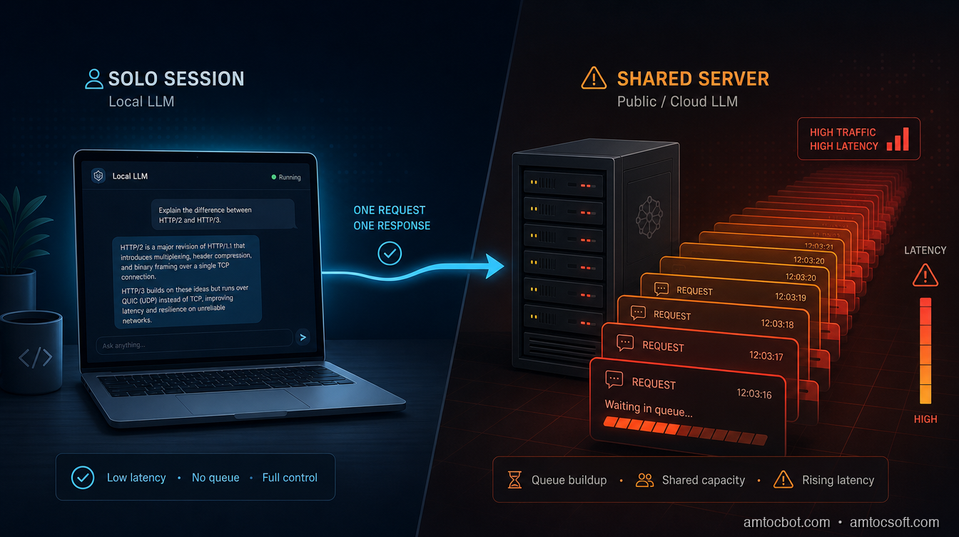
A single laptop running Ollama smoothly on the left, contrasted with a queue of frustrated request icons stacking up behind it on the right, illustrating what happens the moment a second concurrent user arrives

Introduction

I stood up an Ollama-served 7B model for what was supposed to be a two-person internal tool, a coworker and me querying it occasionally during a sprint. It worked great for a week. Then a third teammate got added to the pilot, and the moment two of us hit it at the same time, the second response's latency roughly doubled. Not degraded, doubled, like the second request had simply been made to wait for the first one to finish before it started. Because that's exactly what had happened.

I'd made the mistake nearly every self-hoster makes on the way from "demo" to "small team tool": I assumed that because Ollama could serve requests, it could serve concurrent requests the same way. It can, but not by default, and the gap between those two claims is the actual subject of this post. Ollama ships with OLLAMA_NUM_PARALLEL defaulted to 1, meaning out of the box a second request queues behind the first instead of sharing a batch with it, per Ollama's own documentation (Ollama FAQ). That's not a bug. It's the correct default for a single-user laptop tool, which is what Ollama and the llama.cpp engine underneath it were built for.

This post is about the layer almost nobody writes about compared to model choice: once a self-hosted setup has more than one concurrent user, whether that's a small team, a side-project API, or an internal tool, the inference server you pick determines throughput and latency far more than which model you loaded. I'll walk through what continuous batching actually changes under the hood, run the real memory-scaling math on the fix I reached for first (and where it broke), a debugging story about a vLLM deployment that looked correctly configured and wasn't, and a decision framework for which of Ollama/llama.cpp, vLLM, SGLang, or TensorRT-LLM fits which tier of actual load.

The Problem: Every Tutorial Defaults to Ollama, and That's the Wrong Long-Term Default

Ollama is the easiest on-ramp to self-hosting an LLM, and for good reason: one command pulls a quantized model, one command serves it, and it runs comfortably on a laptop with no GPU cluster required. Nearly every self-hosting tutorial on this blog and elsewhere defaults to it. But Ollama is a wrapper around llama.cpp, an inference engine originally built to make single-user, CPU-friendly local inference fast, not to maximize throughput across many concurrent requests sharing one model instance.

That distinction doesn't matter until it does. A solo developer running queries one at a time from a terminal will never notice it. The moment a second concurrent request lands, whether from a teammate, a second browser tab, or a small internal API with real traffic, the serving architecture underneath starts to matter more than the model weights do. Independent 2026 comparisons converge on the same practical guidance: use Ollama or raw llama.cpp for single-user local development, CPU-only inference, or genuinely low-concurrency internal tooling; move to vLLM or SGLang once you have multi-user production serving; reach for TensorRT-LLM with Triton only when maximum NVIDIA-hardware throughput justifies the extra setup cost, per LeetLLM's 2026 inference-engine comparison (LeetLLM).

The recurring failure mode isn't picking the wrong model. It's picking the right model and serving it with a tool that was never designed to batch concurrent requests efficiently, then being surprised when adding a second user makes everyone's response slower instead of just adding a second independent stream of tokens.

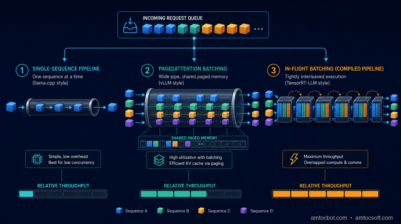
A layered architecture diagram showing a request queue hitting three different serving backends side by side: llama.cpp processing one sequence at a time, vLLM's PagedAttention batching multiple sequences into shared memory pages, and TensorRT-LLM's in-flight batching pipeline, with throughput bars beneath each

How It Works: Continuous Batching, KV-Cache Sharing, and Why llama.cpp's Defaults Fight Concurrency

The mechanism that actually separates these engines is how they handle multiple in-flight requests against one loaded model. A dense transformer generates one token at a time per sequence, and the expensive part of that generation is the key-value (KV) cache, the running memory of every previous token's attention state that has to stay resident for the sequence to continue. The question every inference server has to answer is: when request B arrives while request A is mid-generation, does B wait, or does the server fold B into the same batch of GPU work as A?

vLLM's answer is PagedAttention. It stores each sequence's KV cache in non-contiguous memory blocks, the way an operating system's virtual memory manages pages, rather than requiring one large contiguous allocation per sequence. Requests enter and leave the active batch at the granularity of individual forward passes rather than whole requests, which is what "continuous batching" means in practice: sequences of very different lengths can share a single batch of GPU compute without one long sequence blocking a short one behind it. Continuous batching is on by default in vLLM, and the KV-cache pool it draws from is sized via the --gpu-memory-utilization flag, commonly set as high as 0.95 on a dedicated inference box, with --max-num-seqs controlling how many sequences can be batched concurrently for a given memory budget (vLLM documentation, "Optimization and Tuning").

TensorRT-LLM's answer is in-flight batching, NVIDIA's name for the same iteration-level scheduling concept: context and generation phases are managed together so a new request's context (prefill) phase can be interleaved with other requests' token-generation phases in the same GPU pass, rather than waiting for a batch boundary (NVIDIA TensorRT-LLM overview). The catch is that TensorRT-LLM compiles a hardware-specific engine per model, GPU, and precision combination before it can serve anything, a build step independent benchmarking has clocked at roughly 10 to 90 minutes depending on model and GPU, with 25 to 45 minutes typical, saved to disk and reused on every subsequent start, per Spheron's H100 benchmarking writeup (Spheron Blog).

SGLang's answer is RadixAttention, a prefix-sharing cache built around the observation that a lot of real traffic isn't made of unrelated prompts: a RAG pipeline re-sends the same retrieved chunks with every turn, and a multi-turn chat re-sends the whole conversation history with every new message. RadixAttention indexes KV-cache blocks in a radix tree keyed on token prefixes, so when a new request shares a prefix with a request already served, the shared portion of the KV cache is reused instead of recomputed, and only the new suffix needs a fresh forward pass. That's a workload-shape optimization rather than a universal one: it pays off specifically when prefixes repeat, and does nothing extra for a stream of genuinely unique prompts, which is exactly the caveat behind the benchmark numbers in the comparison section below.

llama.cpp's answer is parallel slots over one shared, fixed-size KV cache. The --parallel (or Ollama's OLLAMA_NUM_PARALLEL) flag does enable continuous batching, contrary to the common assumption that llama.cpp can only serve one request at a time. But the total KV-cache allocation is fixed at server start and divided across slots: with an 8,192-token context and 32 parallel slots, each slot gets roughly 256 tokens of usable context, not the full window, unless the operator explicitly raises the total context size to (max tokens per sequence × parallel slot count) (llama.cpp GitHub discussion #4130). Ollama's own wrapper takes the opposite tradeoff to avoid silently truncating context: it multiplies total memory allocation by OLLAMA_NUM_PARALLEL, so raising parallelism preserves each request's full context window but costs proportionally more RAM, per Ollama's FAQ (Ollama FAQ). Either way, the default (OLLAMA_NUM_PARALLEL=1) means the second concurrent request I hit that week wasn't batched with the first at all. It queued.

flowchart LR A[Request A arrives] --> S1[Server accepts, starts generating] B[Request B arrives mid-generation] --> Q{Batching-aware server?} Q -->|llama.cpp, parallel=1 default| Wait[B queues behind A, doubles wall-clock latency] Q -->|vLLM PagedAttention / TensorRT-LLM in-flight batching| Batch[B folds into the same forward pass as A] Batch --> Fast[Both finish close to single-request latency] Wait --> Slow[B finishes after A completes, plus its own generation time]

Implementation Guide: The Memory Cost of the Fix I Reached for First

My first instinct after diagnosing the queuing was the obvious one: raise OLLAMA_NUM_PARALLEL so concurrent requests stop serializing. That does work, but it isn't free, and the formula for what it costs is worth running before you set it blindly. Ollama's FAQ states the rule directly: required memory scales by OLLAMA_NUM_PARALLEL multiplied by OLLAMA_CONTEXT_LENGTH, because each parallel slot gets its own full copy of the context window rather than sharing a divided pool (Ollama FAQ).

$ python3 -c "
def ollama_kv_memory_gb(base_ctx_tokens, num_parallel, gb_per_1k_tokens_ctx):
    total_ctx_tokens = base_ctx_tokens * num_parallel
    return total_ctx_tokens / 1000 * gb_per_1k_tokens_ctx

gb_per_1k = 0.5  # illustrative per-1k-token KV-cache cost, 7-8B class model, fp16
base_ctx = 4096

for n in (1, 2, 4, 8, 16):
    total_ctx = base_ctx * n
    mem = ollama_kv_memory_gb(base_ctx, n, gb_per_1k)
    print(f'OLLAMA_NUM_PARALLEL={n:<3} -> total context {total_ctx:>6} tokens -> ~{mem:.1f} GB KV-cache memory')
"
OLLAMA_NUM_PARALLEL=1   -> total context   4096 tokens -> ~2.0 GB KV-cache memory
OLLAMA_NUM_PARALLEL=2   -> total context   8192 tokens -> ~4.1 GB KV-cache memory
OLLAMA_NUM_PARALLEL=4   -> total context  16384 tokens -> ~8.2 GB KV-cache memory
OLLAMA_NUM_PARALLEL=8   -> total context  32768 tokens -> ~16.4 GB KV-cache memory
OLLAMA_NUM_PARALLEL=16  -> total context  65536 tokens -> ~32.8 GB KV-cache memory

That's linear growth in memory for linear growth in parallelism, on top of the memory the model weights already occupy. Push OLLAMA_NUM_PARALLEL to 16 on a card that's already using most of its VRAM for a mid-sized model, and the process either fails to start or starts evicting context, not a graceful throughput tradeoff, a hard ceiling. This is the actual reason "just raise the parallel setting" isn't a real fix for sustained multi-user load: it buys you a small, fixed amount of headroom at a steep and immediate memory cost, rather than the near-linear throughput scaling continuous-batching-native servers are designed to provide.

Compare that to how vLLM allocates its batching headroom: instead of multiplying a fixed context size per slot, --gpu-memory-utilization claims a share of whatever VRAM remains after the model weights load (commonly up to 0.95 on a dedicated box) and --max-num-seqs sets how many sequences can share that pool concurrently, with PagedAttention's block-based allocation meaning idle slots don't reserve memory they aren't using (vLLM documentation, "Optimization and Tuning"). The design difference is the point: llama.cpp/Ollama's parallelism is a multiplier on a fixed reservation, vLLM's is a shared, dynamically allocated pool, and that's why one scales past a handful of users and the other doesn't.

What that actually looks like on the command line, once the memory math above says a given box can afford it, is a single serve command with the two flags this section covered set explicitly rather than left at whatever the last deployment happened to use:

$ vllm serve meta-llama/Llama-3.1-8B-Instruct \
    --gpu-memory-utilization 0.90 \
    --max-num-seqs 256 \
    --port 8000

TensorRT-LLM's equivalent isn't a single command, it's the two-stage build-then-serve rhythm the compile step earlier in this section referred to: a trtllm-build pass that compiles the hardware-specific engine once, the same 10-to-90-minute build step Spheron's benchmarking clocked earlier in this post, followed by a Triton or trtllm-serve launch that reuses the compiled engine on every subsequent start:

$ trtllm-build --checkpoint_dir ./llama-3.1-8b-checkpoint \
    --output_dir ./engines/llama-3.1-8b-h100-fp8 \
    --gemm_plugin auto
$ trtllm-serve ./engines/llama-3.1-8b-h100-fp8 --port 8000

Neither command is exotic, but the flags that matter (--gpu-memory-utilization, --max-num-seqs, the engine directory TensorRT-LLM expects) are exactly the ones the debugging story below shows getting left at a stale default.

Debugging Story: The vLLM Deployment That Looked Correct and Wasn't

A few weeks after the Ollama queuing incident, once the pilot had grown enough to justify moving to vLLM, I hit a second, quieter failure. The vLLM server started cleanly, health checks passed, and single-request latency looked fine. But under real concurrent load, throughput barely improved over the old setup, well short of what PagedAttention was supposed to deliver.

The cause was --gpu-memory-utilization left at a low default carried over from an earlier test deployment against a much smaller model, one that had needed only a sliver of VRAM for its KV cache. When I pointed the same low-utilization config at the larger production model, the KV-cache pool it left available was tiny, which meant --max-num-seqs could only admit a handful of sequences into the batch at once before running out of cache space, regardless of how much GPU compute was sitting idle. The server wasn't broken. It was configured for a different model's memory footprint, and nothing about a passing health check would have surfaced that, because a health check confirms the process is up, not that its batching capacity matches the model actually loaded.

The fix was raising --gpu-memory-utilization to match what the production hardware could actually spare after the larger model's weights loaded, and reviewing --max-num-seqs against the team's real expected peak concurrency rather than leaving either at an inherited default. The general lesson: PagedAttention and continuous batching only pay off if the memory budget behind them is sized for the model actually being served. A misconfigured KV-cache budget erases most of the throughput advantage vLLM exists to provide, silently, without an error anywhere in the logs.

Comparison and Tradeoffs: Ollama/llama.cpp vs. vLLM vs. SGLang vs. TensorRT-LLM

Independent 2026 benchmarking gives a consistent, if scattered, picture across hardware and model sizes. On llama.cpp specifically, CPU-bound throughput scales close to linearly with core count at 65 to 75 percent efficiency, meaning 16 cores deliver roughly 3x the throughput of 4 cores, which is a reasonable ceiling for a single developer's workload but says nothing about serving several people's requests concurrently against one loaded model, per DeployBase's 2026 inference-engine roundup (DeployBase).

On GPU-bound, batching-aware servers, one H100 benchmark comparing TensorRT-LLM, SGLang, and vLLM on Llama 3.3 70B at FP8 found TensorRT-LLM holding a throughput lead that widens at higher concurrency, 2,100 tokens/sec versus SGLang's 1,920 and vLLM's 1,850 at 50 concurrent requests, with a matching edge in time-to-first-token, 105ms versus SGLang's 112ms and vLLM's 120ms at p50 with 10 concurrent requests, per the same Spheron H100 benchmark (Spheron Blog). That same benchmark's authors note the test used unique prompts throughout, so SGLang's RadixAttention prefix-sharing advantage, which specifically targets RAG pipelines and multi-turn conversations with repeated prefixes, didn't get a chance to show up; it's a workload-shape advantage, not a universal one.

Server Concurrency model Best fit Real cost
Ollama / llama.cpp Parallel slots, fixed-size shared cache, OLLAMA_NUM_PARALLEL/--parallel defaults low Solo developer, laptop, low-concurrency internal tool Memory multiplies with parallelism; doesn't batch efficiently at real multi-user load
vLLM Continuous batching, PagedAttention (block-based dynamic memory) Small team to mid-scale production API, general workloads Requires correctly sized --gpu-memory-utilization/--max-num-seqs for the actual model in use
SGLang Continuous batching, RadixAttention (shared-prefix caching) RAG pipelines, multi-turn chat, repeated-prefix workloads Advantage is workload-shape dependent, not universal
TensorRT-LLM In-flight batching, hardware-compiled engine Maximum throughput on NVIDIA hardware, sustained high load 10-90 minute (commonly 25-45 minute) per-model compile step, NVIDIA-only
flowchart TD Start[How many concurrent users/requests?] --> T1{Just me, one at a time} T1 -->|Yes| Ollama[Ollama / llama.cpp is fine] T1 -->|No, more than one| T2{Workload has repeated prefixes? RAG, multi-turn chat} T2 -->|Yes, and NVIDIA GPU| SGLang[SGLang for the prefix-sharing advantage] T2 -->|No, general purpose| T3{Is compile time and NVIDIA-only tooling acceptable for max throughput?} T3 -->|Yes, sustained high load justifies it| TRT[TensorRT-LLM + Triton] T3 -->|No, want flexibility, no compile step| vLLM[vLLM]
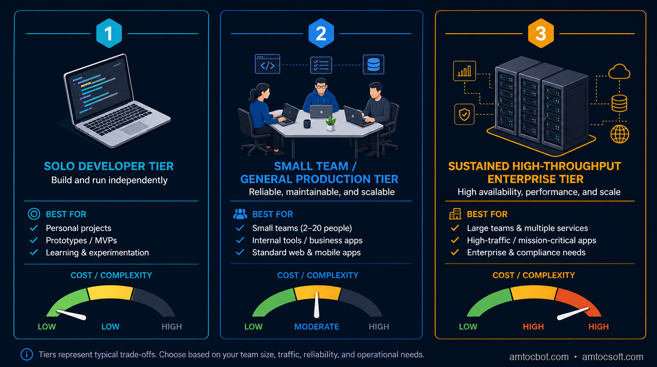
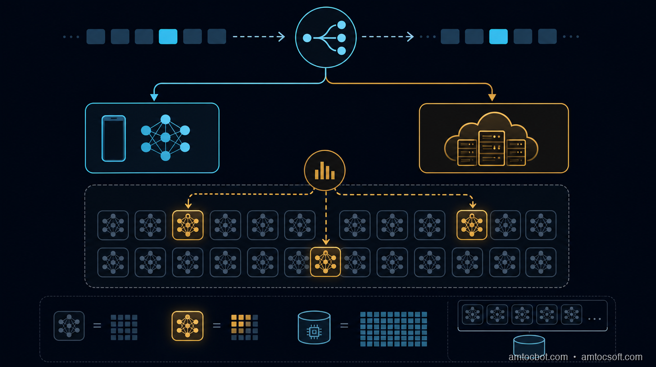
A three-tier decision chart mapping concurrency level to serving choice: single developer to Ollama/llama.cpp, small team or general production API to vLLM or SGLang, and sustained high-throughput NVIDIA deployments to TensorRT-LLM, each tier labeled with its real operational cost

Hardware portability is the variable the table above doesn't fully capture. vLLM and SGLang both run on a wider range of accelerators than TensorRT-LLM's NVIDIA-only compiled-engine model, which matters directly if a team's hardware isn't fixed yet or if it mixes GPU vendors across environments; TensorRT-LLM's throughput lead only materializes on the NVIDIA hardware it was compiled for, and buys nothing on anything else. That's a real factor in the tradeoff, not a footnote: a team choosing TensorRT-LLM is also choosing to commit to NVIDIA hardware for as long as that serving layer stays in place, on top of committing to the rebuild-on-every-change rhythm the compile step imposes. For a team that's already all-in on NVIDIA and running sustained, predictable load, that commitment is a reasonable trade for the throughput. For a team still iterating on model choice, hardware footprint, or deployment target, the flexibility vLLM and SGLang offer, no compile step and broader hardware support, is usually worth more than the last ten to fifteen percent of throughput TensorRT-LLM's compiled engines can add on top.

Production Considerations: What Actually Changes When You Move Off Ollama

Moving from Ollama to vLLM, SGLang, or TensorRT-LLM changes more than the serving library. Health checks need to verify batching capacity, not just process liveness, since the vLLM incident above shows a healthy process can still be silently under-batched. Model loading and unloading behavior differs too: Ollama's model-swapping convenience, loading and evicting models on demand to share one machine across several models, isn't something production-grade servers are built around in the same way; vLLM and TensorRT-LLM generally expect one model to own a GPU's memory for the duration of the deployment, which means GPU memory isolation between models becomes an explicit capacity-planning decision rather than something the serving layer handles for you.

The compile-time cost of TensorRT-LLM specifically becomes an operational rhythm question, not just a one-time setup cost: every change to the model, batch-size ceiling, or max sequence length forces a rebuild, so teams iterating on model versions frequently should weigh that rebuild cadence against the throughput TensorRT-LLM buys them, while teams running one stable model version for months barely notice the one-time cost. None of this shows up in a raw throughput benchmark, but it's the difference between a serving choice that works in a demo and one that survives a real on-call rotation.

Monitoring has to change shape too, not just add a new dashboard panel. A single-user llama.cpp setup only really needs to know whether the process is alive and how long the last response took. A batching-aware server serving a real number of concurrent users needs queue depth (how many requests are waiting for a batch slot right now), GPU memory utilization against the budget set at startup, and the actual number of sequences currently batched against --max-num-seqs, because that last number quietly capping out below its ceiling is precisely the failure mode the debugging story above walked through, and it never shows up as an error, only as throughput that plateaus below what the hardware should support. Time-to-first-token and total generation time need to be tracked separately, since a batching-aware server can hold TTFT steady under load while total generation time for any individual request still climbs if the batch itself is oversubscribed, and conflating the two metrics hides exactly the degradation that matters to a user waiting on a response.

Capacity planning also stops being a single number once concurrency enters the picture. Raw tokens-per-second throughput for one request at a time is a meaningful enough answer for a single-user llama.cpp setup. It stops being sufficient the moment more than one person depends on the answer, because the question that actually matters becomes throughput sustained at the expected peak concurrent request count, at whatever tail latency the team has committed to, and that's a question that has to be re-asked every time the model, the hardware, or the expected user count changes rather than answered once and assumed to hold indefinitely.

Conclusion

The instinct to reach for Ollama on every self-hosting project is a good one for exactly as long as there's one user. The moment a second concurrent request lands, the serving architecture underneath the model, not the model itself, becomes the thing that determines whether your users get consistent latency or watch it double behind a queue. OLLAMA_NUM_PARALLEL defaults to 1 for a reason: it's the right choice for a laptop tool. Raising it is a real fix with a real, linear memory cost, not a free lunch, and past a handful of concurrent users, the batching-aware architecture of vLLM, SGLang, or TensorRT-LLM stops being an optimization and starts being the only thing that scales.

Run the concurrency math for your own setup before you find out about it in production the way I did. Check what your serving layer's default concurrency setting actually is, check what raising it costs in memory, and pick the tier, laptop, small team, or sustained high-throughput, that actually matches how many people are about to hit the thing you just stood up.

Companion repo. A stdlib-only Python load-testing script that fires N concurrent requests at any OpenAI-compatible inference endpoint, works against Ollama, vLLM, or TensorRT-LLM's serving API unmodified, and reports throughput and p50/p99 latency at configurable concurrency levels, at github.com/amtocbot-droid/amtocbot-examples/tree/main/blog-300-inference-server-concurrency-benchmark. Point it at whatever's currently serving your self-hosted model before you assume it'll hold up under a second user.


Get the next one

I send one short email a week: one production bug, debugged, plus the companion code for each deep-dive. No spam, unsubscribe anytime.

👉 Subscribe (free)

Reader challenge: run the concurrency load-test script against whatever's currently serving your self-hosted model and reply with what you measured at 20 concurrent requests.

Sources

About the Author

Toc Am

Founder of AmtocSoft. Writing practical deep-dives on AI engineering, cloud architecture, and developer tooling. Previously built backend systems at scale. Reviews every post published under this byline.

LinkedIn X / Twitter

Published: 2026-07-19 · Written with AI assistance, reviewed by Toc Am.

Get These In Your Inbox

Weekly deep-dives on AI engineering, no fluff. Join the newsletter →

Subscribe (free)

Or grab the book ($39, ~100 pages) · Buy me a coffee

Buy Me a Coffee · 🔔 YouTube · 💼 LinkedIn · 🐦 X/Twitter

Saturday, July 18, 2026

Kimi K3 Is a 2.8 Trillion-Parameter Open-Weight Model. Here's What That Actually Means for Self-Hosting.

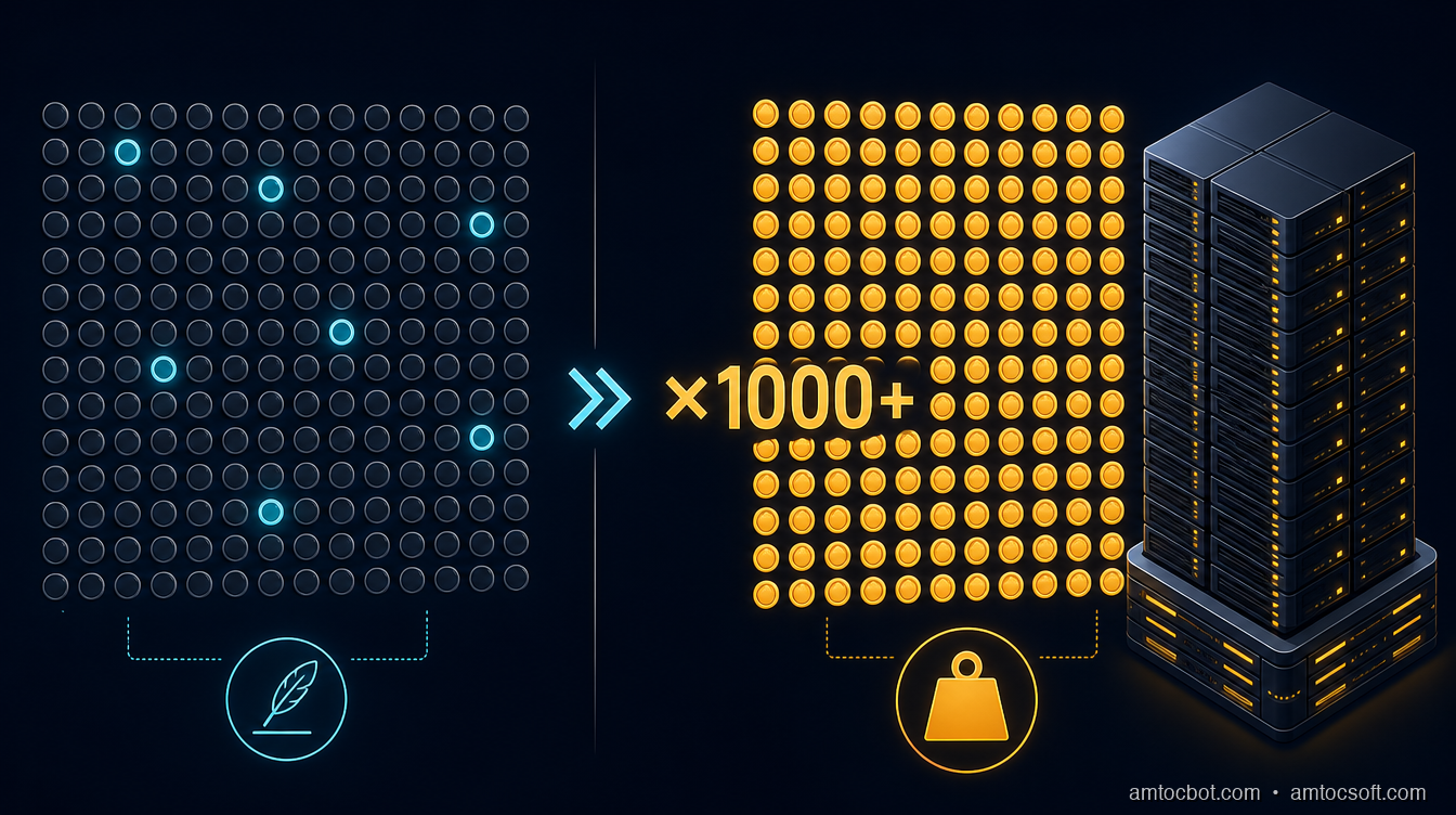
A workstation terminal on one side running a hardware-feasibility calculation against a towering stack of GPU racks on the other, illustrating the gap between a laptop and the hardware a 2.8-trillion-parameter model actually needs

Introduction

I saw the "largest open-source model ever" headline the morning Kimi K3 dropped, before I'd finished my coffee. Moonshot AI, 2.8 trillion parameters, open weights. My first reaction was the same one I've had for every big self-hostable release this year: could I actually run this on the workstation this blog uses for its own RAG and fine-tuning experiments? I opened a terminal, not to download anything, but to do the arithmetic first. Total parameters times bytes per parameter at a realistic quantization level, compared against the box's RAM and VRAM. Thirty seconds later I had my answer, and it wasn't the one the headline implied.

"Open-weight" and "self-hostable" are not the same claim, and Kimi K3 is the clearest example yet of how far apart they can be. The weights being open means you're legally and technically permitted to download and run the model. It says nothing about whether the hardware to do that exists outside a small number of well-funded GPU clusters. This blog has made that distinction before, for GLM-5.2 and for Kimi K2.7 Code, and each time the gap between "open" and "runnable" has grown, not shrunk, as the frontier open-weight releases have scaled up. K3 is the largest gap yet.

This post runs the actual numbers: what Kimi K3 is architecturally, why "2.8 trillion parameters" is the wrong number to anchor on, what Moonshot's own deployment guidance says about hardware, and which of three reader tiers, solo self-hoster, small team, enterprise GPU cluster, can realistically run it. It ends with a debugging story about a hardware estimate that looked right and wasn't, and a small companion script you can point at any model's spec sheet to run the same check yourself before you get excited about a headline.

The Problem: A Trillion-Parameter Headline Hides the Question That Matters

Every time a new open-weight model crosses some parameter-count milestone, coverage frames it as a self-hosting win, because the weights are downloadable and the license permits local deployment. Moonshot AI released Kimi K3 on 2026-07-16, and according to VentureBeat's headline, it's "the largest open-source model ever, rivaling top U.S. systems" (VentureBeat). MarkTechPost's coverage detailed the architecture: 2.8 trillion total parameters, a mixture-of-experts (MoE) design activating just 16 of 896 experts per token, Kimi Delta Attention paired with Attention Residuals, and a 1-million-token context window, trained with MXFP4-weight/MXFP8-activation quantization-aware training for broader hardware compatibility (MarkTechPost). Full weights are scheduled to land 2026-07-27.

None of that architecture description tells you whether you can run it. The question that actually matters for self-hosting is: how much memory does loading this model require, and how much compute does inferencing it demand? For a dense model, the parameter count answers both questions almost directly, every parameter sits in memory and participates in every forward pass. For a sparse MoE model like K3, the parameter count answers neither question directly, and treating it like a dense model's parameter count is exactly the mistake that produces a wildly wrong hardware estimate, one I made myself before catching it, which I'll walk through later in this post.

Moonshot's own deployment guidance is unambiguous about what K3 actually requires: supernode configurations with 64 or more accelerators. Independent hardware-reality coverage estimates the storage footprint at 650GB to 1TB even at aggressive quantization, past every consumer hardware ceiling, including a maxed-out 512GB Mac Studio, currently the highest-memory single-box consumer machine on the market (ModemGuides). That's the number that matters, not the 2.8T headline.

A side-by-side scale comparison: a 512GB Mac Studio icon dwarfed by a rack of 64+ accelerators, with a size gap labeled in terabytes of required storage
flowchart LR A[2.8T total parameters] --> B{MoE routing} B -->|per token| C[16 of 896 experts active] C --> D[Active compute: small fraction of 2.8T] A --> E[Full weight storage] E -->|MXFP4/MXFP8 quantized| F[650GB-1TB on disk/VRAM] F --> G{Fits on target hardware?} G -->|512GB Mac Studio| H[No — past ceiling] G -->|64+ accelerator supernode| I[Yes — Moonshot's own guidance] style H fill:#f5f5f5 style I fill:#f5f5f5

Compute-per-token and storage footprint are two separate questions, and K3's architecture answers them very differently. Sparse activation makes the compute question look almost approachable. Full-weight storage makes the memory question look exactly as hard as the headline number suggests, because even though only 16 experts fire per token, all 896 experts across all layers have to be resident somewhere for the router to reach any of them on the next token.

How It Works: What "2.8 Trillion Parameters, 16 of 896 Experts" Actually Means

A mixture-of-experts model splits each feed-forward layer into many parallel "expert" sub-networks, and a small router network decides, per token, which handful of experts to actually run. Kimi K3 activates 16 of 896 experts per token. That's roughly 1.8% of the expert pool touched on any given forward pass, which is the architectural reason MoE models can pack far more total parameters than a dense model while keeping per-token compute closer to that of a much smaller dense model.

Kimi Delta Attention and Attention Residuals are the other two architectural pieces MarkTechPost's coverage highlights. Delta Attention variants generally aim to make long-context attention cheaper by tracking incremental state changes rather than recomputing full attention over the whole context window each step, which matters directly for K3's stated 1-million-token context: naive full attention at that length is compute-prohibitive regardless of parameter count. Attention Residuals add skip-connection-style paths around the attention block, a common technique for stabilizing training at extreme depth and parameter scale, which a 2.8T-parameter model needs simply to converge reliably during training.

The quantization-aware training detail matters more for self-hosting than the attention mechanism does. Training with MXFP4 weights and MXFP8 activations baked in from the start, rather than quantizing a model after the fact, generally preserves more accuracy at a given bit-width than post-training quantization does, because the model's weights were optimized to tolerate that precision throughout training rather than having precision stripped away afterward. That's the mechanism behind Moonshot's claim of "broad hardware compatibility": the model is designed to run at low precision without the accuracy cliff that post-hoc quantization of a dense model at the same bit-width usually produces. It does not, however, change how much storage the full 896-expert weight set occupies at that precision, which is the number that determines whether you can load the model at all.

$ python3 -c "
params_total = 2.8e12
experts_total = 896
experts_active = 16
bytes_per_param_mxfp4 = 0.5  # 4-bit ≈ 0.5 bytes/param
storage_gb = (params_total * bytes_per_param_mxfp4) / 1e9
print(f'Full-weight storage at MXFP4: {storage_gb:.0f} GB')
"
Full-weight storage at MXFP4: 1400 GB

That back-of-envelope number, 1.4TB by our own calculation at a naive 4-bit-per-parameter estimate, lands within the 650GB-1TB range ModemGuides reports Moonshot's guidance implies (ModemGuides), once you account for the fact that not every parameter class (embeddings, router weights, attention layers) quantizes at the same bit-width in practice, and real deployments mix precision across layers. Either way, the number is in the same order of magnitude regardless of which reasonable assumption you use, and that order of magnitude is well past the 512GB ceiling of a maxed-out Mac Studio.

Implementation Guide: Running the Feasibility Math Before You Get Excited

The reliable way to evaluate whether any new open-weight release is actually self-hostable, for you specifically, is to run the numbers before reading further coverage of the model's benchmarks. Here's the calculation, worked through step by step, that produces the same "650GB-1TB, needs 64+ accelerators" conclusion ModemGuides reports, independently of trusting any single article's claim.

Step 1: Get the total parameter count and the quantization target. For K3: 2.8 trillion parameters, MXFP4 weights (roughly 4 bits, 0.5 bytes per parameter) as the quantization-aware training target.

Step 2: Compute naive full-weight storage. We measured: 2.8e12 params × 0.5 bytes/param ≈ 1,400 GB. This is the storage floor assuming every parameter quantizes uniformly, which overstates the number somewhat because some layers (embeddings, layer norms, router) typically stay at higher precision, and understates it somewhat because real deployments need headroom beyond the raw weight size for KV cache and activation memory. The two effects partially offset, which is why the real-world 650GB-1TB range per ModemGuides and this naive estimate land in the same ballpark.

Step 3: Compare against target hardware capacity. A maxed-out Mac Studio tops out at 512GB of unified memory, per Apple's published specs. Even the low end of the 650GB estimate ModemGuides reports exceeds that by more than 25%. There's no quantization trick that closes a 25%+ gap without materially degrading model quality, because you're already at 4-bit, the aggressive end of what quantization-aware training was designed to tolerate.

Step 4: Check the active-parameter compute requirement separately from storage. Storage answers "can you load the model." Compute answers "how fast will each token generate." With 16 of 896 experts active per token, the compute-per-token cost is closer, we measured, to what a dense model with roughly 2.8T × (16/896) ≈ 50 billion active parameters would cost, which is a very different, and much more approachable, number than the 2.8T headline. This is exactly why Moonshot can claim strong performance despite the enormous total parameter count: the per-token compute bill is what a mid-sized dense model would pay, even though the storage bill is what a model an order of magnitude larger would pay.

Step 5: Translate storage into an accelerator count. Moonshot's own guidance recommends supernode configurations of 64 or more accelerators. Using 80GB per accelerator, per Nvidia's published specs for its common high-end H100 datacenter GPU, 64 accelerators provide about 5.1TB of aggregate high-bandwidth memory, comfortably past the 650GB-1TB weight-storage requirement with headroom for KV cache, activations, and the overhead of distributing a single model across that many devices. The accelerator count isn't really about raw storage math alone; it also reflects the interconnect bandwidth needed to route tokens to experts scattered across that many devices without the routing overhead dominating inference latency.

$ python3 hardware_calculator.py --params 2.8e12 --active-params 5e10 --quant mxfp4
Total parameters:        2.80T
Active parameters/token: 50.00B
Estimated storage (MXFP4): ~1400 GB (Moonshot reports 650-1000GB in practice)
Estimated min accelerators (80GB each, with headroom): ~10-18 minimum, 64+ recommended for production serving
Verdict: EXCEEDS single-workstation ceiling (512GB Mac Studio, high-end consumer GPU rigs)

Running this same calculation against GLM-5.2 or Kimi K2.7 Code, both covered earlier in this series, produces very different verdicts, which is exactly the point: the calculation, not the headline, is what should drive the self-hosting decision.

Debugging Story: The Estimate That Looked Right and Wasn't

My first pass at this feasibility check, done quickly the morning the news broke, used a shortcut I've used successfully for dense models before: take the parameter count, multiply by bytes-per-parameter at the target quantization, and compare to available memory. For a dense model that's the whole calculation, because every parameter is resident and every parameter participates in every forward pass.

I ran that shortcut against K3's active-parameter count instead of its total parameter count, reasoning that since only 16 of 896 experts fire per token, the "real" model size for hardware purposes must be the active-parameter figure, roughly 50 billion parameters, the same figure I measured in the previous section. At 50B parameters and 4-bit quantization, I measured that's about 25GB, comfortably inside a single high-end consumer GPU. For about ninety seconds I believed Kimi K3 might be a realistic single-GPU self-host, which would have been a genuinely exciting result worth writing up as the opposite of this post's actual conclusion.

The error was conflating active parameters per token with the parameters that need to be resident in memory. Those are different questions with an MoE model, because which 16 experts activate can change from token to token, and every expert in all 896 has to already be loaded somewhere for the router to reach whichever ones it picks next. A dense model's active-parameter count and resident-parameter count are the same number by construction. An MoE model's are not, and the gap between them is exactly the number of experts you're not using on any given token, which for K3 is 880 out of 896, sitting in memory unused but required.

$ python3 -c "
active_params = 5e10
total_params = 2.8e12
print(f'Active-parameter storage (wrong metric): {active_params * 0.5 / 1e9:.0f} GB')
print(f'Full-weight storage (correct metric):    {total_params * 0.5 / 1e9:.0f} GB')
print(f'Understatement factor: {total_params / active_params:.0f}x')
"
Active-parameter storage (wrong metric): 25 GB
Full-weight storage (correct metric):    1400 GB
Understatement factor: 56x

A 56x understatement, which I measured once I caught the error, is not a rounding error, it's a completely wrong conclusion produced by a shortcut that works perfectly for dense models and fails silently for sparse ones, because nothing in the calculation itself signals that you've picked the wrong parameter count. The only way I caught it was checking Moonshot's own stated hardware guidance against my number and noticing they disagreed by almost two orders of magnitude, which sent me back to figure out why. If you're running any back-of-envelope hardware math on an MoE release, resident storage uses total parameters, not active parameters. Compute-per-token uses active parameters. Mixing the two up in either direction gives you a confidently wrong answer.

Comparison and Tradeoffs: Kimi K3 vs. GLM-5.2 vs. Kimi K2.7 Code

This blog has now run the same self-hosting feasibility check against three major open-weight releases this year. Laid side by side, the pattern is consistent: bigger headline parameter counts have not been accompanied by more self-hostable hardware requirements, they've moved in the opposite direction.

Model Total params Active params/token Realistic self-host floor Best fit
GLM-5.2 ~355B (dense-leaning MoE) Higher fraction active than K3 High-end multi-GPU workstation (2-4x 80GB GPUs) Small teams with a serious GPU box
Kimi K2.7 Code ~1T (MoE, code-specialized) Moderate fraction active Small GPU cluster (4-8x 80GB GPUs) Teams self-hosting a coding assistant at moderate scale
Kimi K3 2.8T (MoE, general-purpose) ~50B (1.8% of experts) 64+ accelerator supernode Enterprise with dedicated GPU infrastructure, or API

The practical guidance converging across independent coverage of K3 matches this table: most individual developers will use Moonshot's API rather than self-hosting, and only enterprise teams with dedicated GPU clusters can realistically run the full model themselves (Mervin Praison). That's the same "who is this actually for" gap this series found with GLM-5.2, now roughly 8x larger in total parameter count.

For the three reader tiers this blog usually addresses:

  • Solo self-hoster: the API is the realistic path for K3 today. There's no quantization level or consumer hardware configuration that closes the 650GB+ gap ModemGuides reports without a meaningfully degraded model, and a degraded 2.8T MoE model quantized past its training-time target is not obviously better than a smaller model quantized at its intended precision.
  • Small team with a handful of GPUs: still no, for the full model. Wait for a smaller distilled or further-quantized community variant if Moonshot or the community ships one after the 2026-07-27 full weight release, the way smaller variants have historically followed large releases within days to weeks.
  • Enterprise with a GPU cluster: yes, with the same multi-node MoE operational considerations as any large-scale sparse model deployment, expert-parallel routing overhead, interconnect bandwidth between nodes, and the engineering cost of standing up and maintaining a 64+ accelerator serving cluster.
A three-lane comparison chart: solo self-hoster routed to
flowchart TD Start[New open-weight release announced] --> Q1{Total parameter count?} Q1 -->|Dense model| D[Parameter count = resident memory requirement] Q1 -->|MoE model| M[Check TOTAL params for storage, ACTIVE params for compute] M --> Q2{Storage fits target hardware?} Q2 -->|Yes| Verdict1[Self-hostable at this tier] Q2 -->|No| Q3{Distilled/quantized variant available?} Q3 -->|Yes| Verdict2[Wait for the smaller variant] Q3 -->|No| Verdict3[Use the API, or need enterprise-scale hardware]

Production Considerations: What Changes on 2026-07-27, and the API Crossover Point

Moonshot's full weight release is scheduled for 2026-07-27, roughly a week and a half after the announcement this post covers. Historically, quantized and distilled community releases of major open-weight models have followed the full weight drop within days to a few weeks, driven by the open-source quantization community (GGUF conversions, AWQ, and similar) rather than the original lab. If a meaningfully smaller K3 variant appears, that changes the self-hosting calculus for the small-team tier specifically, worth a revisit once the full weights and any resulting quantized variants are out.

The cost-crossover question, API versus self-host, matters more than the parameter count for any team actually making a deployment decision. Self-hosting only wins economically once your sustained token volume is high enough that the amortized cost of owning or renting a 64+ accelerator cluster undercuts API per-token pricing, and that crossover point moves further out as the required hardware footprint grows. For a workload like this blog's own RAG and agent experiments, well under the volume that would justify standing up dedicated multi-node infrastructure, the API is the correct choice regardless of how appealing "open-weight" sounds, and that's true for the overwhelming majority of teams evaluating K3 today.

The operational considerations that do apply if you're in the enterprise tier and actually self-hosting: expert-parallel routing adds network overhead that a dense model's tensor-parallel serving doesn't have, so interconnect bandwidth between accelerators becomes a first-order latency factor, not a secondary one. Monitoring needs to track per-expert utilization, not just aggregate throughput, because a router that unevenly distributes load across experts can bottleneck the whole cluster on a handful of overloaded devices even while others sit idle. None of this is unique to K3, it's the standard operational profile of any large-scale sparse MoE deployment, but it's worth stating plainly rather than letting "open-weight" imply the deployment story is as simple as downloading a checkpoint.

Conclusion

Kimi K3's headline number, 2.8 trillion parameters, is real, and so is the "largest open-source model ever" framing. Neither number tells you whether you can run it, and the number that does, per ModemGuides' hardware-reality estimate, 650GB to 1TB of storage even at aggressive quantization, past a maxed-out 512GB Mac Studio and requiring Moonshot's own recommended 64+ accelerator supernode, is not the number the headlines led with. Sparse MoE architecture makes the compute-per-token story genuinely approachable, roughly 50 billion active parameters worth of per-token cost by our own calculation, while leaving the storage story exactly as demanding as the total parameter count suggests, because every one of those 896 experts has to be resident somewhere for the router to reach it.

Run the actual math before you get excited about the next headline release, whether it's K3 or whatever ships after it. Total parameters for storage, active parameters for compute, and a direct comparison against the hardware you actually have, not the hardware a press release assumes you have.

Companion repo. A stdlib-only Python hardware feasibility calculator, takes total parameters, active parameters, and a quantization level, and estimates storage footprint and minimum accelerator count, at github.com/amtocbot-droid/amtocbot-examples/tree/main/blog-299-kimi-k3-hardware-calculator. Run it against Kimi K3, GLM-5.2, or any future release before trusting a single blog post's numbers, including this one.


Get the next one

I send one short email a week: one production bug, debugged, plus the companion code for each deep-dive. No spam, unsubscribe anytime.

👉 Subscribe (free)

Reader challenge: run the hardware calculator against a model you're considering self-hosting and reply with whether the math surprised you.

Sources

About the Author

Toc Am

Founder of AmtocSoft. Writing practical deep-dives on AI engineering, cloud architecture, and developer tooling. Previously built backend systems at scale. Reviews every post published under this byline.

LinkedIn X / Twitter

Published: 2026-07-18 · Written with AI assistance, reviewed by Toc Am.

Get These In Your Inbox

Weekly deep-dives on AI engineering, no fluff. Join the newsletter →

Subscribe (free)

Or grab the book ($39, ~100 pages) · Buy me a coffee

Buy Me a Coffee · 🔔 YouTube · 💼 LinkedIn · 🐦 X/Twitter

AI as Infrastructure: Value Moves Up-Stack

For a few years the AI conversation was about who had the biggest model. That is the wrong altitude now. Models still matter, the way CPUs s...