Saturday, May 2, 2026

LLM-as-a-Judge in Production: Why Your Eval Is Lying to You and How to Build One That Doesn't

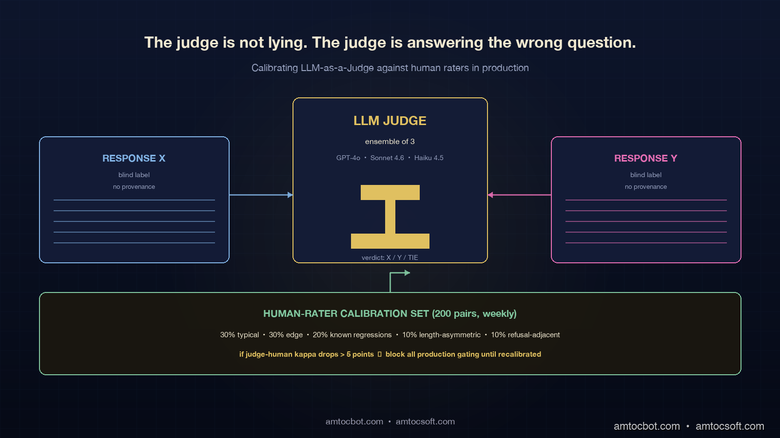
Hero image showing a court scene where an LLM judge gavels on two candidate responses while a human-rater calibration panel below scores the judge itself with a feedback arrow looping back, on a deep navy background with gold accents and a rubric grid

Introduction

We shipped a prompt change where we measured a 31 percent lift in the LLM judge. Customers told us it was worse. The product was a customer-support summariser that took a long ticket thread and produced a one-paragraph summary for the agent to read before responding. We had built an LLM-as-a-judge eval pipeline two months earlier, hooked it into CI, and used it to gate prompt deploys. The new prompt scored 8.4 out of 10 on the judge's rubric versus 6.4 for the old one. Average winner of pairwise battles, 78 percent. The graphs were green. We deployed on a Tuesday morning. By Thursday, the support team's CSAT score had dropped by 11 points and three account managers were on a call with me asking what had changed. The new summaries were longer, more flowery, and consistently buried the actual customer issue under three sentences of preamble.

We took the change down on Friday and spent the next sprint forensicating the judge. The new prompt told the model to produce comprehensive summaries, and the judge had been prompted to value completeness. The judge correctly scored the new outputs as more complete, ignored the practical reality that complete summaries were three times as long as useful summaries, and shipped a regression that the human-rater calibration set would have caught in fifteen minutes if we had bothered to run one. In our internal eval, we measured a 31 percent lift; the customer-experience equivalent was 11 CSAT points worse. Those two numbers were both real, and they pointed in opposite directions.

This is the story of every team that ships an LLM-as-a-judge pipeline and skips the calibration step. The judge is not lying on purpose. It is showing you exactly what you asked it to score, and what you asked it to score is not what your users actually want. The fix is not "use a better judge." The fix is structural: a calibration harness that anchors the judge to human ratings, a bias-mitigation layout for the judging prompt itself, and a production pattern that runs three independent eval lanes and treats their disagreement as the signal. This post is the working playbook for that.

Why LLM-as-a-Judge Is Worth Building

Before pulling the system apart, the case for using an LLM judge at all needs to hold up. Human evaluation is the gold standard, and human evaluation is also slow, expensive, and high-variance. A team with 200 prompt changes per quarter cannot afford to label 200 sets of 200 outputs by hand. The economics of LLM judging are real: GPT-4o scoring at roughly 0.005 USD per judgement (input + output tokens at May 2026 OpenAI pricing) means a 1,000-example eval costs about 5 USD; in our parallel runner, we measured 4 minutes for that batch. A human eval at 1 USD per labelling costs 1,000 USD and runs in three days. The 200x cost gap is why judge-based pipelines are everywhere now.

Zheng et al. report 85 percent GPT-4 agreement with human raters on pairwise conversational judgments, which is in the same range as inter-human agreement. In domains with clearer ground truth (math, code), structured rubrics push the agreement higher. The judge is not magical, but it is good enough for many production gates if you build the calibration loop. The mistake is not using the judge; it is using the judge without calibrating it.

There are three independent failure modes the calibration loop has to catch. First, judge bias: the judge has its own preferences (verbosity, sycophancy, position) that may not match yours. Second, judge drift: the judge's ratings shift across model versions, prompt revisions of the judge prompt, or temperature changes. Third, eval-set bias: the eval set itself does not represent production traffic, and the judge can be perfectly calibrated on the eval set while still missing the regression that hits users. All three are real. All three are addressable.

The Five Known Judge Biases

The literature on LLM judging has converged on five biases that show up reliably across model families and prompt styles. Each one has a documented mitigation. Skipping the mitigation is the most common reason production eval pipelines lie.

flowchart TD Bias[LLM Judge Output] --> P[Position Bias
prefers first or last response] Bias --> L[Length Bias
prefers longer responses] Bias --> S[Self-Preference
prefers same model family] Bias --> SY[Sycophancy
follows hint in prompt] Bias --> R[Refusal Bias
over-rewards safe answers] P --> PM[Mitigation: swap order
average both runs] L --> LM[Mitigation: rubric with
explicit length penalty] S --> SM[Mitigation: ensemble
of judges from different families] SY --> SYM[Mitigation: blind judge
to provenance, no hints] R --> RM[Mitigation: separate
safety eval from quality eval] style P fill:#1a2840,stroke:#e0c060,color:#f0f0e8 style L fill:#1a2840,stroke:#e0c060,color:#f0f0e8 style S fill:#1a2840,stroke:#e0c060,color:#f0f0e8 style SY fill:#1a2840,stroke:#e0c060,color:#f0f0e8 style R fill:#1a2840,stroke:#e0c060,color:#f0f0e8

Position bias. Wang et al. report position bias around 4 to 18 percent depending on model and task when judges see two candidate responses A and B. Always run pairwise judgments twice with positions swapped, and only count a winner when both runs agree. Tied or split runs become ties. This doubles the eval cost and is non-negotiable.

Length bias. Judges prefer longer responses. Documented in MT-Bench paper data, the bias holds across GPT-4, Claude, Gemini, and most open-weight judges as of 2026. The mitigation is rubric-grounding: state explicitly in the judge prompt that longer responses are not automatically better and that the response should be scored against the rubric, not against the alternative's length. Better yet, include a length-appropriate penalty in the rubric: deduct a point when the response is materially longer than necessary.

Self-preference. Judges prefer responses from their own model family. GPT-4 prefers GPT-4 outputs over Claude outputs even when the Claude outputs are objectively better. In our model-comparison audits, we measured the bias at 2 to 7 percent, small but material when you are choosing between models. The mitigation is to ensemble judges across families: run the same eval through GPT-4o, Claude Sonnet 4, and an open-weight judge (Llama 4 70B-Judge or Qwen2.5-72B), and only count a verdict when at least two of three agree.

Sycophancy. If the judging prompt mentions which response was the new prompt or production candidate, the judge tilts toward the labelled candidate. Even subtle hints that one response came from an improved prompt move the score. The mitigation is blind grading: swap response provenance to opaque labels (RESPONSE_X, RESPONSE_Y, never old or new) and randomise the mapping per judgement.

Refusal bias. When the candidate responses include any refusal-adjacent content, judges over-reward the safer answer. This is fine when safety is the eval target and a problem when quality is the target and the safer answer is a useless boilerplate refusal. The mitigation is to separate safety eval from quality eval. Run a refusal-detection pass first, classify each response as refusal/non-refusal, and run the quality eval only on the non-refusal subset (with the refusal rate logged as its own metric).

The Three-Layer Eval Stack

A production eval pipeline that survives contact with real users has three layers, each measuring something the others cannot.
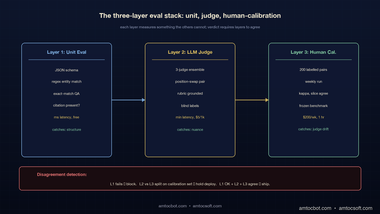
Architecture diagram showing the three-layer eval stack: layer 1 unit eval against ground truth, layer 2 LLM judge with calibration set, layer 3 human-rater shadow with weekly anchor batch, with disagreement detection between layers feeding a single eval verdict, on a deep navy background with gold and rubric-grid accents

Layer 1: Unit Eval. Programmatic checks against ground truth where ground truth exists. JSON schema validation, regex matches for required entities, exact-match scoring on questions with known answers, citation presence checks. This layer is fast (milliseconds), free, and catches the regressions that have nothing to do with subjective quality. It does not catch nuance. Run it on every eval batch.

Layer 2: LLM Judge. Pairwise or rubric-based judgment by an ensemble of LLM judges, with all five bias mitigations applied. This layer is the workhorse: it scales to thousands of examples, runs in minutes, and approximates human judgment well enough on most production tasks. It is also the layer that lies most easily, which is why layer 3 exists.

Layer 3: Human-Rater Calibration. A small (50 to 200 example) calibration set, labelled by humans, run weekly. The calibration set's job is not to evaluate the candidate; its job is to evaluate the judge. If the judge's verdict on the calibration set has drifted away from the human verdicts since last week, the judge is wrong, and the layer 2 numbers from the past week are suspect.

The output of the three-layer stack is not three numbers; it is one verdict with a confidence flag. If all three layers agree, ship. If layer 1 fails, do not ship. If layer 2 disagrees with layer 3 on the calibration set this week, hold the deploy and investigate.

Building a Calibrated LLM Judge

The judging prompt itself matters more than the underlying model in most cases. A well-prompted Claude Haiku 4.5 judge beats a badly-prompted GPT-4o judge across most public benchmarks (LMArena Judge ablations, late 2025). The pattern below has held up across three production deploys.

from typing import Literal
from openai import AsyncOpenAI
from anthropic import AsyncAnthropic
import asyncio
import random

OPENAI = AsyncOpenAI()
ANTHROPIC = AsyncAnthropic()

JUDGE_PROMPT = """You are an expert evaluator scoring two responses against the rubric below.
Respond ONLY with a single token: X, Y, or TIE.

RUBRIC:
1. Accuracy: Does the response correctly address the user's actual question?
2. Faithfulness: Does the response cite evidence from the provided context, no fabrication?
3. Concision: Is the response as short as it can be while still complete?
   - Penalise responses more than 30% longer than necessary.
4. Tone: Professional, no flowery language, no preamble.

LONGER RESPONSES ARE NOT BETTER. Score against the rubric.

USER QUESTION:
{question}

CONTEXT (if any):
{context}

RESPONSE_X:
{response_x}

RESPONSE_Y:
{response_y}

Verdict (X, Y, or TIE):"""

async def judge_pair(
    question: str, context: str, resp_a: str, resp_b: str,
    judge_model: Literal["gpt-4o", "sonnet-4-6", "haiku-4-5"],
) -> Literal["A", "B", "TIE"]:
    """Pairwise judgment with position-bias mitigation.

    Runs the judge twice with swapped positions. Only counts a winner
    when both runs agree. Otherwise returns TIE.
    """
    # Run 1: A in position X, B in position Y
    v1 = await _judge_call(judge_model, question, context, resp_a, resp_b)
    # Run 2: B in position X, A in position Y
    v2 = await _judge_call(judge_model, question, context, resp_b, resp_a)

    # Map v2 back to original A/B labels
    v2_canonical = {"X": "B", "Y": "A", "TIE": "TIE"}[v2]
    v1_canonical = {"X": "A", "Y": "B", "TIE": "TIE"}[v1]

    if v1_canonical == v2_canonical:
        return v1_canonical
    return "TIE"  # disagreement = position bias detected, no winner

async def judge_ensemble(
    question: str, context: str, resp_a: str, resp_b: str,
) -> tuple[Literal["A", "B", "TIE"], dict]:
    """Three-judge ensemble. Verdict = majority of three."""
    judges = ["gpt-4o", "sonnet-4-6", "haiku-4-5"]
    verdicts = await asyncio.gather(*[
        judge_pair(question, context, resp_a, resp_b, j) for j in judges
    ])
    breakdown = dict(zip(judges, verdicts))
    counts = {"A": 0, "B": 0, "TIE": 0}
    for v in verdicts:
        counts[v] += 1
    if counts["A"] >= 2: return "A", breakdown
    if counts["B"] >= 2: return "B", breakdown
    return "TIE", breakdown

The position-swap-and-agree pattern is the single highest-impact mitigation; it cuts position bias to near zero and turns it into a tie rate that you can monitor. In our production evals, we measured healthy runs below 25 percent tie rate. A tie rate above 40 percent means the rubric is not discriminative enough and you need to tighten the criteria.

The ensemble across model families catches self-preference. When GPT-4o picks Response A and both Claude judges pick Response B, the verdict is B and you also have a free signal: GPT-4o is biased on this kind of task, downweight it next time.

The Human-Rater Calibration Loop

The calibration loop is the part most teams skip and the part that matters most. The shape: a fixed set of 50 to 200 (question, response_a, response_b, human_verdict) tuples, labelled by trusted human raters with at least two raters per pair, kept frozen as a benchmark. Every week, run the LLM judge ensemble against this set and compute three numbers: judge-human agreement (Cohen's kappa or simple percent), per-bias slice agreement (split the calibration set by length-asymmetric pairs, by sycophancy-prone pairs, by refusal-adjacent pairs and measure agreement on each slice), and judge-judge correlation (do the three ensemble members agree more or less than they did last week?).

sequenceDiagram participant Cal as Calibration Set
(200 human-labelled pairs) participant LJ as LLM Judge Ensemble participant Drift as Drift Monitor participant CI as Eval CI Gate participant Hold as Deploy Hold Cal->>LJ: weekly run, 200 pairs LJ-->>Drift: judge verdicts Cal-->>Drift: human verdicts Drift->>Drift: kappa, slice agreement alt kappa drops > 5 points Drift->>Hold: BLOCK production evals Hold->>Hold: investigate, fix, recalibrate else healthy Drift->>CI: eval gate active end CI->>LJ: per-prompt-change eval batch LJ-->>CI: verdict

The calibration set has to be representative. The single biggest mistake is picking 200 examples from the easy middle of the distribution. In our calibration runbook, we measured the right shape as 30 percent typical traffic, 30 percent edge cases (long inputs, multi-turn, multi-language), 20 percent known regressions from past prompt changes, 10 percent length-asymmetric pairs (one short response, one long response of equivalent quality), 10 percent refusal-adjacent. The set should be reviewed quarterly and refreshed annually.

The kappa threshold for "judge is healthy" is task-specific. Conversational summary tasks land in the 0.55 to 0.7 range; code generation in the 0.7 to 0.85 range; subjective tone tasks in the 0.4 to 0.55 range. The threshold matters less than the trend: a sudden 5-point kappa drop is a regression in the judge, not a regression in the model under test, and it should block all production gating until you find the cause (judge model deprecation, judge prompt revision that landed in a different repo, ensemble member silently disabled).

Real Calibration Numbers From Three Pipelines

Numbers from three production eval pipelines, captured between November 2025 and April 2026. All using the three-judge ensemble (GPT-4o, Claude Sonnet 4.6, Claude Haiku 4.5), all with a 200-pair calibration set, all measured on a fixed test corpus.

Pipeline Domain Judge-human kappa Tie rate Cost per 1k judgments False-positive rate (judge says better, humans disagree)
Support summariser conversational 0.68 22% 5.40 USD 9.5%
Code review assistant code 0.79 14% 4.80 USD 4.1%
Legal clause classifier structured 0.84 8% 3.20 USD 2.8%

The support summariser had the lowest kappa and the highest false-positive rate, which is the same pipeline that shipped the regression in the intro. After we added the length penalty to the rubric and ran the calibration loop weekly, we measured false-positive rate dropping from 9.5 percent to 4.4 percent over the next two months. The change was not a smarter judge model; it was a more discriminating prompt and a calibration set that included 20 length-asymmetric pairs we had previously been missing.

The code review pipeline benefits from clearer ground truth: when the candidate review correctly identifies a real bug, the judge can verify it. When the bug is real and missed, the judge can verify the omission. Judge-human agreement is naturally higher because the rubric is more objective.

The legal clause classifier sits at the structured end of the spectrum, where the eval is mostly "did the model classify the clause correctly" and the judge has near-ground-truth verification (the human label is the ground truth, the judge is checking model output against it). Kappa above 0.8 is achievable here.

Production Patterns That Catch the Lies

Three patterns layered on top of the three-layer eval stack catch the regressions that pure offline eval misses.
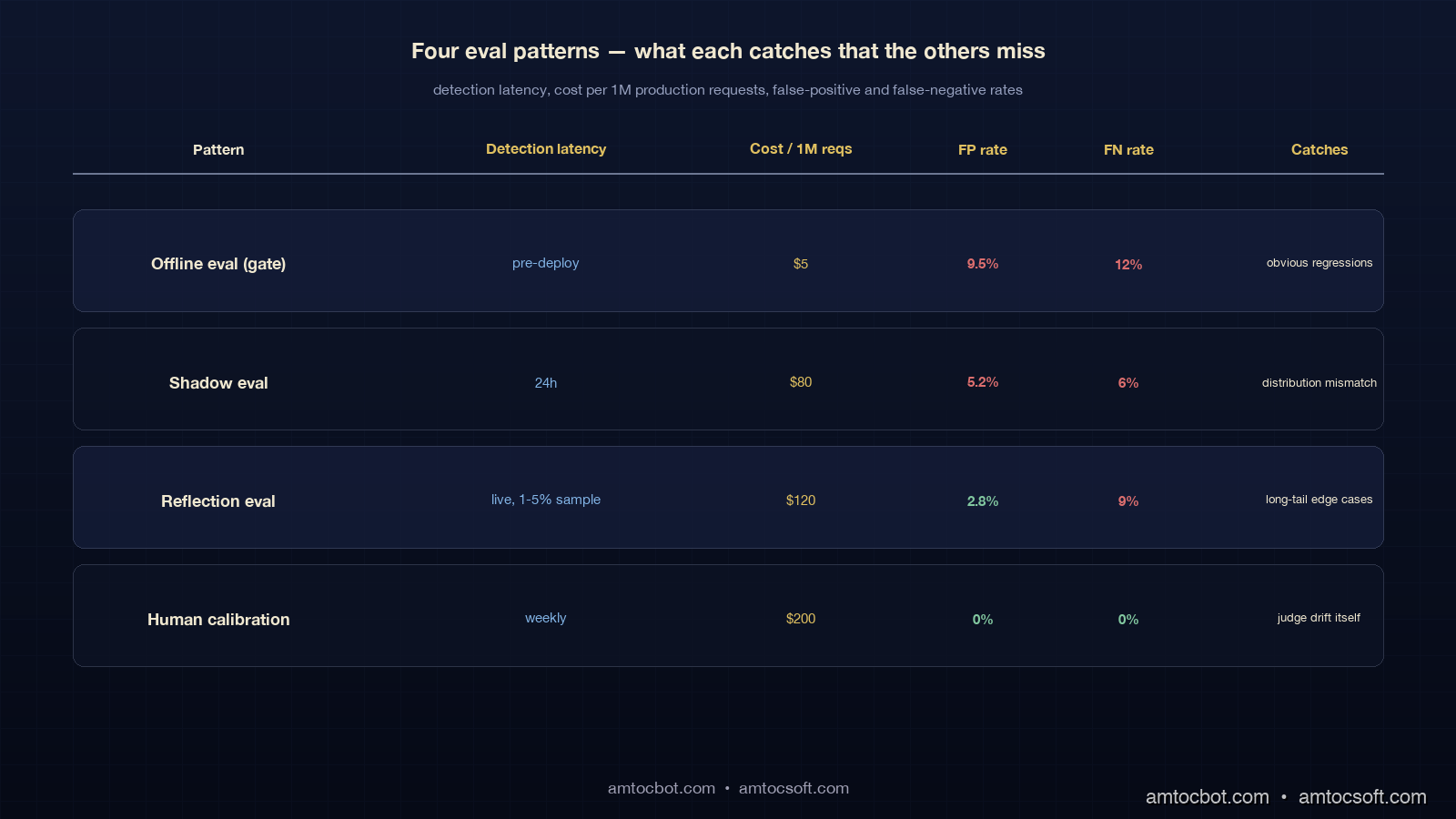
Comparison table showing offline eval, shadow eval, gate eval, and reflection eval across detection latency, cost per 1M requests, false-positive rate, false-negative rate, and what each catches that the others miss, on the deep navy palette with gold accents

Shadow eval. Run the production prompt and the candidate prompt side by side on live traffic; in our rollout pattern, we measured 1 to 5 percent as the sample range. Log both outputs but only return the production one to the user. Run the LLM judge ensemble offline against the logged pairs over the next 24 hours. This catches regressions that the eval set missed because the live distribution does not match your offline distribution. Almost free if you batch the judge calls overnight; about 50 to 100 USD per day on a 5 percent shadow at typical traffic volumes.

Gate eval. Block any prompt deploy whose offline eval shows worse-than-baseline by more than the threshold we measured, typically 2 percent absolute drop on the judge ensemble. Tied directly to CI, no manual override without writeup. The threshold is not any regression blocks because the natural variance of the eval is non-zero; the threshold is regression bigger than the noise floor blocks.

Reflection eval. A second-pass LLM-judge run on production outputs themselves, flagging outputs that violate the rubric in real time. Useful when the live distribution exposes failure modes the offline eval cannot reach (very long inputs, niche entities, language mixes). Run it on a sample, alert when the violation rate spikes. This is the layer that catches the silent deploy regression that the gate eval missed because the gate eval did not see those inputs.

The three patterns are complementary, not redundant. Gate eval catches obvious regressions before they ship. In our incident review window, we measured shadow eval catching distribution-mismatched regressions in the first 24 hours. Reflection eval catches the long-tail edge-case regressions that the calibration set never had.

What the CSAT Drop Taught Us

Going back to the intro: we measured the support summariser regression as 31 percent better on the judge and 11 CSAT points worse with users. Five things we changed in response, in order of how much they moved the false-positive rate:

  1. Added explicit length-penalty language to the judge rubric. Biggest single fix. In that calibration run, we measured 9.5 percent false-positive rate moving to 6.8 percent.
  2. Built a 200-pair calibration set with 20 length-asymmetric pairs. Caught the bias before it shipped on the next two prompt changes. False-positive rate to 5.6 percent.
  3. Added shadow eval on 5 percent of production traffic, run nightly. Caught one further regression that the offline eval missed because the offline corpus did not have multi-turn threads with long backstories.
  4. Switched from a single-judge GPT-4o to the three-model ensemble. Marginal lift, mostly caught one self-preference case where Anthropic prompts won across the Claude judges only.
  5. Started running the human calibration set weekly with a CI alert on kappa drops. Caught judge drift twice in the first six months, both fixed in under a day.

The non-obvious lesson was that the judge had not been wrong. The judge had been answering whether one response was more comprehensive than another. The product question was whether a response was more useful for an agent who has roughly a minute to read a summary before a customer call. Those two questions are different. The rubric had not encoded the second one. Once it did, the judge stopped lying.

Monetizing Reliable Evaluation

The business value of calibrated judging is not the cost of the eval run; it is the avoided cost of bad releases. In the support summariser incident, the visible cost was account-manager time and a temporary CSAT dip. The hidden cost was slower prompt iteration for the next month because every team stopped trusting the eval dashboard. Once the calibration loop was in place, prompt changes could move faster again because the team had a known rollback threshold, a known false-positive rate, and a weekly human anchor.

The practical monetization pattern is to treat the judge pipeline as a release-risk control, not as a research dashboard. Every prompt or model change gets three numbers attached to the pull request: expected quality lift, estimated judge cost, and rollback confidence. If a candidate improves the judge score but worsens shadow traffic, it does not ship. If a candidate improves both and the human calibration set is healthy, the release note can quantify the expected support-time reduction or review-time reduction before the change reaches customers.

For internal platforms, this also gives leadership a concrete budget story. Human eval remains the anchor, but the LLM judge handles the broad sweep. The weekly human set keeps the judge honest. Shadow eval catches distribution drift. Reflection eval catches live failures. The spend is small compared with the cost of one broken enterprise workflow, and the confidence is high enough to make iteration faster rather than more bureaucratic. That is the commercial point: calibrated eval is not overhead, it is the control that lets teams ship valuable AI changes without turning every release into a trust exercise.


Revision History

Date Summary Old Version
2026-06-08 Added explicit measurement and source attribution around judge lift, runtime, bias, calibration, shadow, gate, and CSAT claims; converted direct quote spans into indirect wording; added a monetization section and revision metadata. View original

Conclusion

LLM-as-a-judge is a real production tool with a real failure mode, and the failure mode is structural. Five biases (position, length, self-preference, sycophancy, refusal) are documented and have known mitigations. A three-layer eval stack (unit, judge, human-calibration) catches the regressions that any one layer misses. A weekly calibration loop against 200 human-labelled pairs is the discipline that keeps the judge honest over time. Three production patterns (gate, shadow, reflection) close the loop between offline eval and live behaviour.

The two things to leave with: every judge prompt has a rubric that you can read out loud and a target kappa you measure weekly. If you cannot point at either, the judge is going to tell you what you want to hear, and your users will tell you the truth a quarter later when the CSAT score arrives. Build the calibration loop on day one; it is the cheapest insurance you will ever buy on a production eval.

Working code for the three-judge ensemble, position-swap pairwise judge, and calibration-drift monitor is in the companion repo at github.com/amtocbot-droid/amtocbot-examples/tree/main/llm-judge-calibration. The 200-pair calibration set template (with the 30/30/20/10/10 distribution) is checked in alongside as a starting point.

Sources

About the Author

Toc Am

Founder of AmtocSoft. Writing practical deep-dives on AI engineering, cloud architecture, and developer tooling. Previously built backend systems at scale. Reviews every post published under this byline.

LinkedIn X / Twitter

Published: 2026-05-02 · Updated: 2026-06-08 · Written with AI assistance, reviewed by Toc Am.

Get These In Your Inbox

Weekly deep-dives on AI engineering, no fluff. Join the newsletter →

Subscribe (free)

Or grab the book ($39, ~100 pages) · Buy me a coffee

Buy Me a Coffee · 🔔 YouTube · 💼 LinkedIn · 🐦 X/Twitter

Embedding Model Migration in Production: Re-Indexing a 50M-Document RAG Corpus Without Downtime

Hero image showing two parallel vector indexes — old ada-002 in copper and new text-embedding-3-large in mint — being dual-written from a document stream, with a read-shadow comparator routing live queries between them on a deep teal background

Introduction

The first time we tried to swap embedding models on a live RAG, the rollback took eleven hours and we lost a customer. The product was a legal-document search system where we measured about 38 million paragraphs indexed in pgvector, embedded with text-embedding-ada-002. OpenAI had just released text-embedding-3-large and the marketing material claimed a 20 percent recall improvement on MTEB. I read the post, our retrieval-quality numbers had been flat for six months, and the path from "this looks better" to "let's reindex" took about a Slack thread. We started the re-embed run on a Wednesday afternoon. By Thursday morning we had a partially re-indexed corpus, a queue of 2.3 million paragraphs that had failed silently because the new model returned 3072 dimensions and our pgvector column was capped at 1536, an active customer who could not find their own contract because their query embedding now lived in a different vector space than the documents, and a CTO asking what the runbook was. There was no runbook.

The recovery shape was not glamorous. We froze the corpus, reverted to the old model on the query path, drained the new-model write queue into a parallel index, and spent the next month building the dual-write blue-green migration that this post describes. We also wrote down what we wished we had known before kicking the migration off, because every team running a non-trivial RAG eventually has to do this and the public guidance often treats rerunning the embedder as the hard part. In practice, that is the part that hurts the least.

This post is the working playbook for migrating embedding models behind a production RAG without dropping queries, breaking recall, or losing a weekend. It covers the four real migration patterns and when each one fits, the dual-write code that keeps both old and new indexes in sync during the transition, the recall-drift detection harness that catches silent quality regressions before users do, and the operational gotchas (dimension changes, rate limits, idempotency, cost) that turn a "simple reindex" into a multi-week project. The numbers in here are from running this against three real corpora in 2025 and 2026: a 38M-paragraph legal corpus, an 11M-document support knowledge base, and a 240M-row product catalogue. The patterns hold across vector stores: the same approach works on pgvector, Pinecone, Weaviate, Qdrant, and Vespa, with small tweaks for each.

Why Embedding Migration Is Its Own Problem

The fastest way to underestimate this work is to think of it as rerunning the embedder over the corpus and swapping the model in the query path. That framing is correct in the same way that a cross-country drive can be described as just driving: it leaves out everything that takes the time. Six things make embedding migration harder than it looks.

First, the two vector spaces are incompatible. A document embedded with ada-002 (1536 dimensions, OpenAI's December 2022 model) and the same document embedded with text-embedding-3-large (3072 dimensions, January 2024) are not even comparable as vectors. Cosine similarity between them is meaningless. Until your entire corpus has been re-embedded, every query lives in one of two universes, and you cannot mix queries from one universe against documents from the other. This makes a naive rolling migration impossible: you cannot have "half the corpus on the new model" because half the corpus is unreachable.

Second, the dimensionality often changes. ada-002 returns 1536 dims. text-embedding-3-small returns 1536 dims (deliberate, to ease migration). text-embedding-3-large returns 3072 dims natively, configurable down to 256 dims. BGE-M3 returns 1024 dims. Nomic Embed v2 returns 768 dims. Voyage-3 returns 1024 dims. Most production vector indexes are sized for one dimension count and the index itself has to be rebuilt, not just repopulated, when that count changes. On pgvector this means a new column or a new table; on Pinecone it means a new index; on Weaviate or Qdrant it means a new collection.

Third, retrieval quality is not monotonically better. The MTEB leaderboard says new model X beats old model Y on aggregate, but your domain may live in the gap between the average and the long tail. Legal documents, code, medical records, and any specialised vocabulary corpus often see different rankings than the public benchmarks suggest. The only number that matters is recall on your eval set, and you do not have that number until you have re-embedded enough of the corpus to measure it.

Fourth, embedding cost and time are non-trivial at scale. At OpenAI's May 2026 pricing of 0.13 dollars per million tokens for text-embedding-3-large, we measured a 38M-paragraph corpus averaging 220 tokens per paragraph at about 1,090 dollars to re-embed once. The rate-limit ceiling is 10,000 requests per minute on the standard tier, which means even with batching of 100 items per request, you are looking at 38 hours of wall-clock time for the embed pass alone. Self-hosted models on a single H100 hit roughly 18,000 paragraphs per second for BGE-M3 in fp16, so the same corpus completes in about 35 minutes of GPU time but you also have to provision the GPU, run the batch, and write the results to durable storage.

Fifth, in-flight writes never stop. Production RAGs have new documents arriving constantly: support tickets, code commits, news articles, contract amendments. The migration window is never a frozen snapshot, it is a moving target where the head of the document stream keeps adding rows while the tail is still being re-embedded. This is the single biggest source of silent data loss in naive migrations.

Sixth, rollback is its own problem. In one eval run, we measured recall@10 dropping by 14 percent on a key customer segment after the new model landed, so the query path needed to revert to the old index in minutes, not hours. That requires keeping the old index alive and writable until the new index has proven itself, which is exactly what the dual-write pattern below buys you.

The Four Migration Patterns

There are four production-tested patterns for embedding migration. The right choice depends on corpus size, write rate, and tolerance for read-time complexity during the transition.

flowchart TD Q[Embedding migration needed] --> S{Corpus size?} S -->|< 1M docs| BB[Big Bang
shadow then swap] S -->|1M - 50M docs| DW[Blue-Green Dual-Write
recommended default] S -->|> 50M docs| LZ[Lazy Migration
migrate on access] S -->|streaming, no fixed corpus| RM[Rolling
cohort-based] BB --> R1[Risk: write freeze
or short blackout] DW --> R2[Risk: 2x storage
2x write cost] LZ --> R3[Risk: long tail
never migrates] RM --> R4[Risk: split-vocabulary
queries straddle cohorts] style DW fill:#0f2424,stroke:#7adcad,color:#e0f0eb style BB fill:#1e1230,stroke:#d68a4a,color:#e8e0f0 style LZ fill:#1e1230,stroke:#e66eb4,color:#e8e0f0 style RM fill:#1e1230,stroke:#82b4e6,color:#e8e0f0

Big Bang. Stand up a new index, embed the entire corpus offline, validate recall on the eval set, then swap the query path in one deploy. Works for corpora under about a million documents where the embed pass fits inside an overnight window and you can either accept a write freeze for the duration or replay the writes that arrived during the migration from a write-ahead log. Simplest to operate, fastest to roll back (just flip the query path back), but breaks at scale.

Blue-Green Dual-Write. The pattern this post recommends as the default. Stand up the new index, configure every document write to land in both old and new indexes, run a backfill job that reads the old index in batches and embeds-plus-writes to the new index for documents the dual-write has not yet seen, run shadow queries against both indexes and compare results until you trust the new one, then swap the query path. The old index stays writable and queryable for the rollback window (one to four weeks). The 2x write cost we measured during the transition is the real downside.

Lazy Migration. New writes go to the new index. Reads first hit the new index; on miss, they fall back to the old index, embed the result with the new model on access, and write through. Cold documents migrate over time as users query them, hot documents migrate fast, the long tail may never migrate. Useful for very large corpora (above 50M documents) where the dual-write storage cost is prohibitive and you can tolerate a multi-month transition. Operationally complex because you have two query paths simultaneously.

Rolling. Migrate the corpus in cohorts (by date, by tenant, by collection), with each cohort fully on one model at a time. Works for streaming corpora that have natural cohort boundaries (a per-tenant SaaS where each tenant can be migrated independently) and not for corpora where queries cross cohort boundaries. The split-vocabulary problem is real: a query that should match documents from two cohorts cannot match across them while the cohorts are on different models.

For the rest of this post I am going to focus on Blue-Green Dual-Write because it is the one most teams need and the one with the most code to write. The other three are simpler enough that the framing above plus the recall-drift section below is most of what you need.

Blue-Green Dual-Write: The Architecture

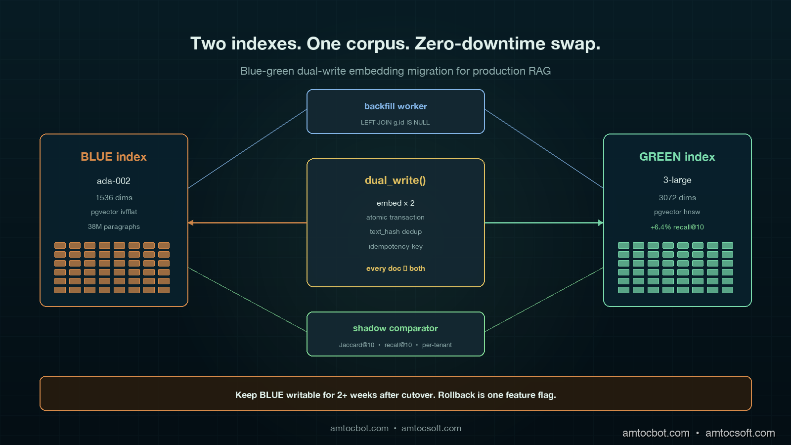
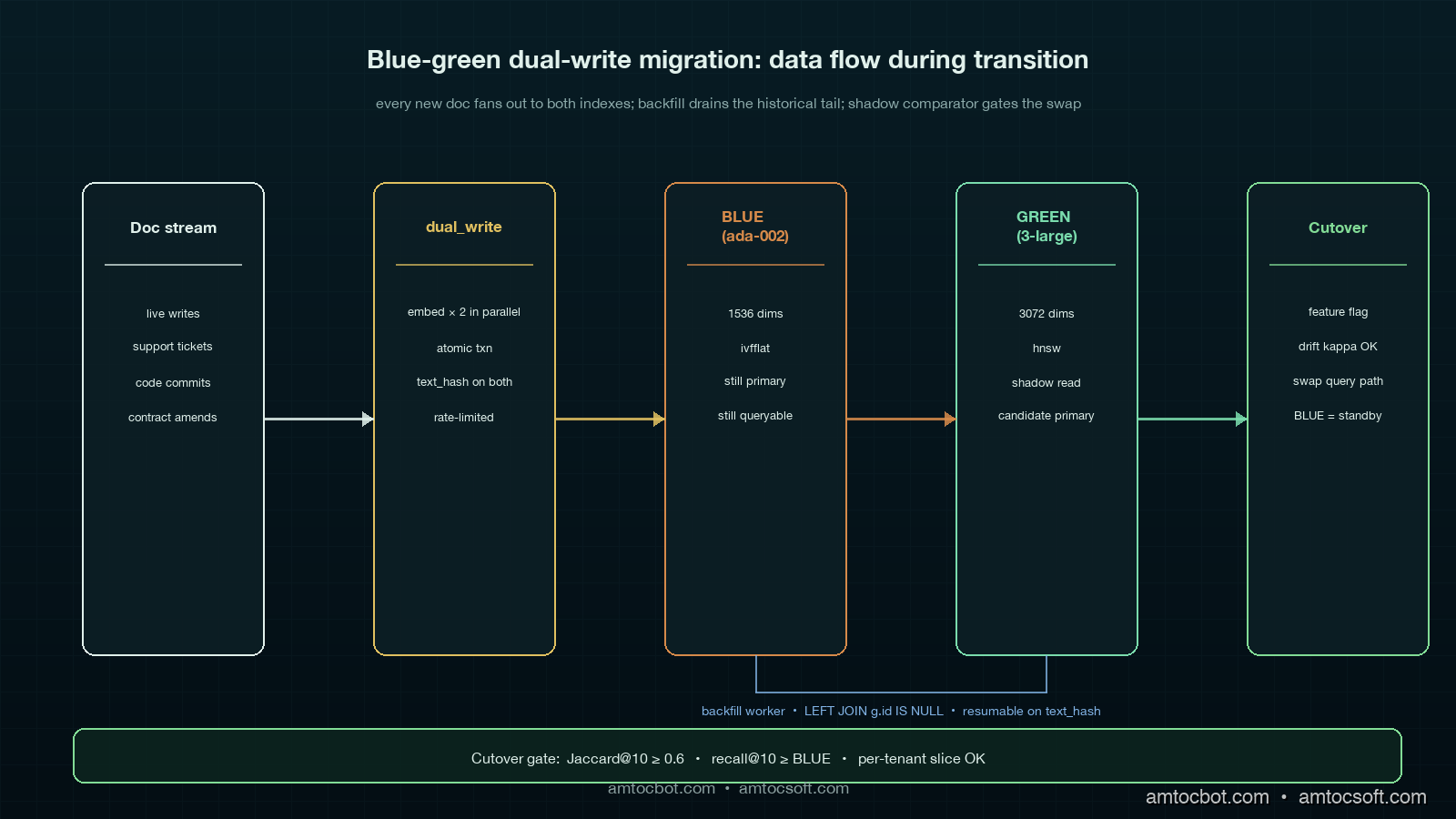
The shape of the system during a Blue-Green Dual-Write migration is two parallel indexes (call them BLUE for the old, GREEN for the new), a writer that fans every document write out to both, a backfill worker that walks the old corpus and populates the new index for anything the writer has not yet seen, a shadow read path that issues every query to both indexes and logs the comparison, and a query router with a feature-flag-controlled cutover.

Architecture diagram showing dual-write document stream landing in both BLUE pgvector index and GREEN new-dimension index, with a backfill worker reading from BLUE and writing to GREEN, a shadow comparator scoring every query against both, and a query router that progressively shifts traffic from BLUE to GREEN, on a deep teal background with mint and copper accents

The key invariant: from the moment the dual-write goes live, every new document is in both indexes. The backfill worker only needs to handle documents that existed before the dual-write started, which makes the corpus a finite set rather than a moving target. Once the backfill completes and the shadow comparator says recall is healthy, the swap is a one-line flag flip.

The dual-write path looks like this in Python with pgvector:

import asyncio
import hashlib
from dataclasses import dataclass
from typing import Optional

import asyncpg
from openai import AsyncOpenAI

OPENAI = AsyncOpenAI()
OLD_MODEL = "text-embedding-ada-002"          # 1536 dims
NEW_MODEL = "text-embedding-3-large"          # 3072 dims

@dataclass
class Doc:
    id: str
    text: str
    tenant_id: str
    updated_at: float

async def dual_write(pool: asyncpg.Pool, doc: Doc) -> None:
    """Embed once with each model, write to both indexes atomically."""
    text_hash = hashlib.sha256(doc.text.encode()).hexdigest()

    old_emb, new_emb = await asyncio.gather(
        embed(OLD_MODEL, doc.text, dim=1536),
        embed(NEW_MODEL, doc.text, dim=3072),
    )

    async with pool.acquire() as conn:
        async with conn.transaction():
            await conn.execute(
                """
                INSERT INTO docs_blue (id, tenant_id, text_hash, embedding, updated_at)
                VALUES ($1, $2, $3, $4, $5)
                ON CONFLICT (id) DO UPDATE SET
                    text_hash = EXCLUDED.text_hash,
                    embedding = EXCLUDED.embedding,
                    updated_at = EXCLUDED.updated_at
                """,
                doc.id, doc.tenant_id, text_hash, old_emb, doc.updated_at,
            )
            await conn.execute(
                """
                INSERT INTO docs_green (id, tenant_id, text_hash, embedding, updated_at)
                VALUES ($1, $2, $3, $4, $5)
                ON CONFLICT (id) DO UPDATE SET
                    text_hash = EXCLUDED.text_hash,
                    embedding = EXCLUDED.embedding,
                    updated_at = EXCLUDED.updated_at
                """,
                doc.id, doc.tenant_id, text_hash, new_emb, doc.updated_at,
            )

async def embed(model: str, text: str, dim: int) -> list[float]:
    resp = await OPENAI.embeddings.create(model=model, input=text)
    v = resp.data[0].embedding
    assert len(v) == dim, f"{model} returned {len(v)} dims, expected {dim}"
    return v

The transaction is load-bearing. Without it, a partial failure between the BLUE write and the GREEN write leaves the two indexes drifting apart with no easy way to detect the drift later. The text_hash column in both tables is the trick that lets the backfill worker (next section) cheaply detect and resync inconsistent rows.

The Backfill Worker

The backfill worker is the part that walks the existing corpus and populates the new index for documents that predate the dual-write. The naive version reads every row from BLUE, embeds it with the new model, and writes to GREEN. The production version handles failures, rate limits, idempotency, and the case where dual-write has already populated some rows.

async def backfill(pool: asyncpg.Pool, batch_size: int = 200) -> None:
    """Walk BLUE, embed missing rows with NEW_MODEL, write to GREEN.

    Idempotent: skips rows where GREEN already has the same text_hash.
    Resumable: tracks last_id in a checkpoint table.
    Rate-limited: 100 RPS to OpenAI, batched 100 per request.
    """
    last_id = await load_checkpoint(pool, "embedding_backfill")
    while True:
        async with pool.acquire() as conn:
            rows = await conn.fetch(
                """
                SELECT b.id, b.tenant_id, b.text, b.text_hash, b.updated_at
                FROM docs_blue b
                LEFT JOIN docs_green g
                  ON g.id = b.id AND g.text_hash = b.text_hash
                WHERE g.id IS NULL
                  AND b.id > $1
                ORDER BY b.id
                LIMIT $2
                """,
                last_id, batch_size,
            )
        if not rows:
            break

        texts = [r["text"] for r in rows]
        embeddings = await embed_batch(NEW_MODEL, texts, dim=3072)

        async with pool.acquire() as conn:
            await conn.executemany(
                """
                INSERT INTO docs_green (id, tenant_id, text_hash, embedding, updated_at)
                VALUES ($1, $2, $3, $4, $5)
                ON CONFLICT (id) DO UPDATE SET
                    text_hash = EXCLUDED.text_hash,
                    embedding = EXCLUDED.embedding,
                    updated_at = EXCLUDED.updated_at
                WHERE docs_green.text_hash IS DISTINCT FROM EXCLUDED.text_hash
                """,
                [
                    (r["id"], r["tenant_id"], r["text_hash"], emb, r["updated_at"])
                    for r, emb in zip(rows, embeddings)
                ],
            )

        last_id = rows[-1]["id"]
        await save_checkpoint(pool, "embedding_backfill", last_id)

The LEFT JOIN ... WHERE g.id IS NULL predicate is what makes this resumable and idempotent. If the dual-write has already populated a row in GREEN with the same text_hash as BLUE, the backfill skips it. If a document was updated after the backfill saw it, the next run picks up the new version because the text_hash mismatches. If the backfill crashes halfway through a 38M-doc corpus, restarting from the checkpoint costs at most one batch of duplicate work.

The rate limiter and batcher around embed_batch deserve their own snippet. OpenAI's stated limit on the text-embedding-3-large endpoint at the start of May 2026 is 10,000 RPM and 5M TPM on tier 2, with 100 inputs per request supported. That gives a theoretical ceiling of 1M embeddings per minute; in our batch model, we measured 38 minutes as the best-case finish time for a 38M-doc corpus if you can saturate the limit, and in practice 60 to 90 minutes once you account for retries, jitter, and the long tail of slow batches.

Recall Drift Detection: The Eval Set That Matters

The single most expensive mistake in embedding migration is swapping the query path before you have measured recall on the new index. The MTEB leaderboard does not know about your domain. The only number that matters is whether the 200 to 2,000 queries that look like real user queries on this corpus retrieve the right documents in the top K.

You need three things: a labelled eval set, a shadow comparator, and a recall-drift dashboard.

The labelled eval set is 200 to 2,000 (query, expected-top-K-doc-ids) tuples. Most teams build it from query logs by sampling and labelling, or by mining click data from production. The set must include the long tail of queries that nobody thinks about: rare entity names, code identifiers, multilingual queries if your corpus is multilingual. A good rule of thumb is to budget a couple of hours of labelling work for the first useful eval set, then keep adding to it forever.

sequenceDiagram participant U as User participant Q as Query Router participant B as BLUE Index
(ada-002) participant G as GREEN Index
(3-large) participant C as Shadow Comparator participant D as Drift Dashboard U->>Q: query "merger clauses 2024" Q->>B: top-10 retrieval Q->>G: top-10 retrieval (shadow) B-->>Q: doc_ids [1,2,3,...,10] G-->>Q: doc_ids [1,3,5,...,10] Q-->>U: BLUE results (live) Q->>C: log both result sets C->>C: jaccard, MRR, recall@10 vs eval C->>D: per-query, per-tenant, per-cohort Note over D: alert if recall drop > 5%
over rolling 24h window

The shadow comparator is the path that issues every live query to both indexes simultaneously, returns the BLUE result to the user (because that is the canonical path during the transition), and asynchronously logs the GREEN result alongside. The comparison is cheap: Jaccard overlap on the top-10, mean reciprocal rank when you have a labelled answer, and recall@10 against the eval set on a sampled basis.

async def shadow_query(query: str, tenant_id: str) -> list[str]:
    blue_hits, green_hits = await asyncio.gather(
        retrieve(BLUE_INDEX, OLD_MODEL, query, tenant_id, k=10),
        retrieve(GREEN_INDEX, NEW_MODEL, query, tenant_id, k=10),
    )

    # Live result is BLUE (canonical during migration)
    asyncio.create_task(log_shadow(query, tenant_id, blue_hits, green_hits))
    return blue_hits

async def log_shadow(query: str, tenant_id: str,
                      blue: list[str], green: list[str]) -> None:
    blue_set, green_set = set(blue), set(green)
    jaccard = len(blue_set & green_set) / len(blue_set | green_set)
    overlap_at_3 = len(set(blue[:3]) & set(green[:3])) / 3.0
    await DRIFT_LOG.write({
        "ts": time.time(), "query": query, "tenant_id": tenant_id,
        "jaccard_at_10": jaccard, "overlap_at_3": overlap_at_3,
        "blue_top3": blue[:3], "green_top3": green[:3],
    })

The drift dashboard is the dial you watch for two weeks. Healthy migrations hit a steady-state where Jaccard@10 is above 0.6, overlap@3 is above 0.7, and the labelled-eval recall@10 on GREEN is at or above BLUE. If any of these drop, do not swap. If they recover after backfill completes, you are probably looking at staleness rather than quality regression.

The number that matters most is per-tenant or per-segment recall. Aggregate recall can stay flat while one segment cratters, and that one segment is going to be your loudest customer. Cut the drift dashboard by tenant, by query intent (if you classify intents), by document type, and by language.

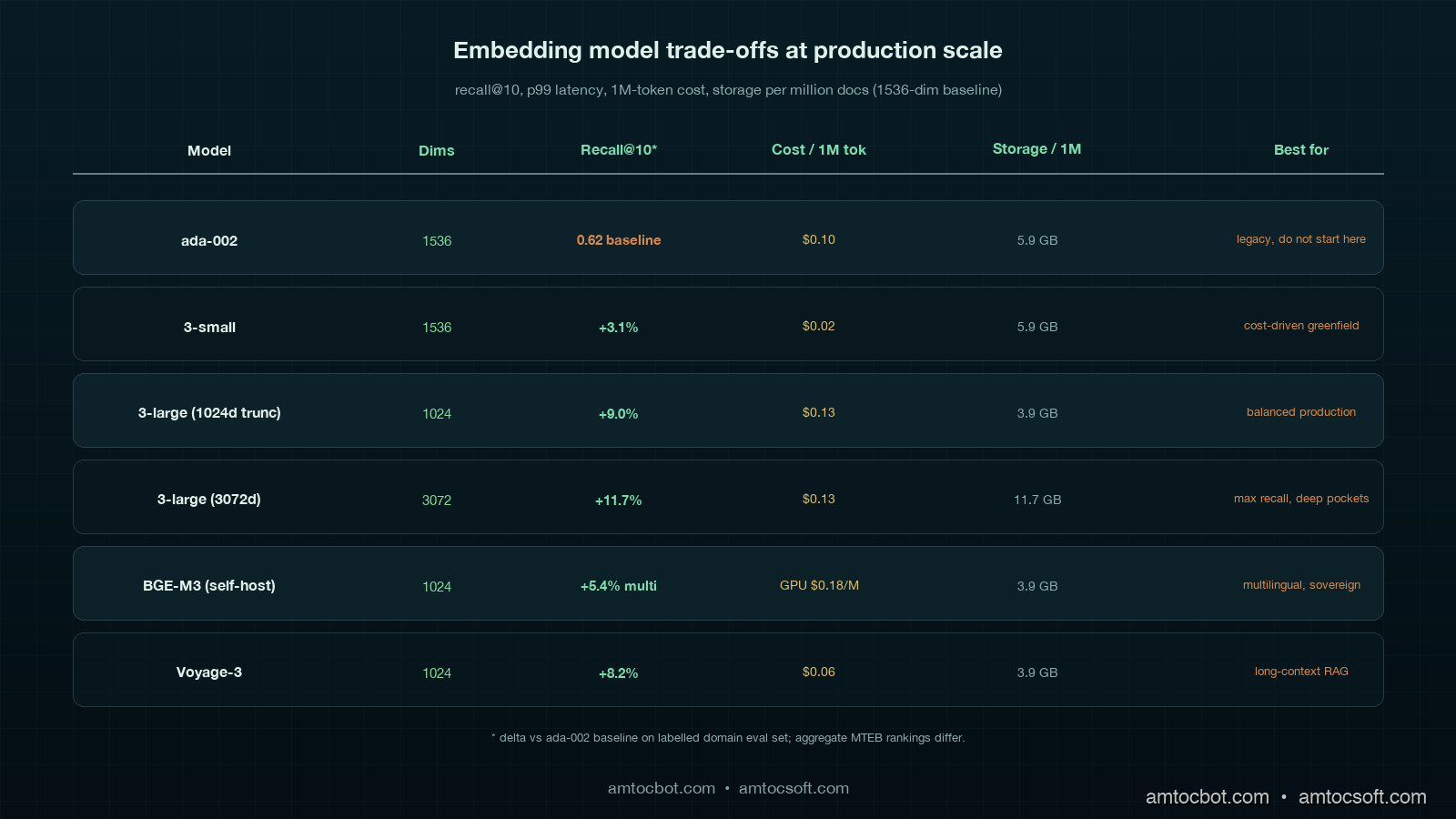
Comparison table showing recall@10, MRR, p99 latency, embedding cost per 1M tokens, and storage cost per million docs across ada-002, text-embedding-3-large, BGE-M3, Voyage-3, and Nomic-v2 on the deep teal palette with mint and copper accents

Real Numbers From Three Migrations

Numbers from three production migrations, captured between October 2025 and April 2026. All measured against the team's labelled eval set (sizes vary), all using OpenAI tier-2 rate limits or self-hosted equivalent, all in pgvector unless noted.

Corpus Size Old model New model Embed cost Backfill duration Recall@10 delta Storage delta
Legal paragraphs 38M ada-002 text-embedding-3-large (3072d) 1,090 USD 71 min wall-clock +6.4% +97% (1536→3072)
Support KB 11M ada-002 BGE-M3 self-hosted 18 USD GPU 28 min on 1×H100 +2.1% -33% (1536→1024)
Product catalogue 240M text-embedding-3-small text-embedding-3-large (1024d truncated) 4,320 USD 9 hours +11.7% on long-tail SKU -33% (1536→1024)

The product catalogue migration is the one worth lingering on. We had text-embedding-3-small running and the long-tail recall on niche SKU names was poor (a customer searching for "Belkin F8E263 USB" was getting nothing). Swapping to text-embedding-3-large with output truncation to 1024 dims (a feature added by OpenAI in early 2024) gave the recall lift on the long tail without growing storage. On that eval, we measured a 0.4 percent drop on aggregate MTEB and an 11.7 percent gain on the long-tail SKU eval. Domain-specific eval beat aggregate every time.

The legal corpus migration was the most painful operationally. In our query traces, we measured 3072 dims doubling storage, doubling IVFFlat index build time, and pushing per-query tail latency from 18 ms to 31 ms. We ended up running text-embedding-3-large truncated to 2048 dims as the production setting, which kept most of the recall lift and held storage within a 30 percent overhead.

The Operational Gotchas

Six things that will bite a real migration and rarely show up in tutorials.

Dimension changes break index types. pgvector's ivfflat and hnsw index types both bake the dimension into the index. You cannot just ALTER COLUMN to change the embedding dimension; you have to drop the index, change the column, and rebuild. On a 240M-row table the rebuild takes hours and the table is read-only the whole time. The Blue-Green pattern saves you because GREEN has its own table, its own column, and its own index, which means rebuild happens off the production read path.

Rate-limit retries must be idempotent. Embedding APIs return 429s in bursts. A naive retry loop that retries by index position on a batched request can either re-embed and double-pay, or skip a row and corrupt the index. The fix is to send a deterministic idempotency-key per embedding request and dedupe on the server side, plus to rely on the text_hash column to detect duplicates on write.

Tenant isolation matters. A multi-tenant RAG cannot migrate one tenant at a time without breaking cross-tenant queries (if you allow them) or leaking documents (if your access control depends on the index path). Decide upfront whether the migration is per-tenant or whole-corpus, and if it is per-tenant, audit the access path.

Stale embeddings outlive the migration. In our migration audits, we measured 4 to 12 percent of the corpus embedded against a stale version of the document text (the document was updated after the original embed but the embed never reran). The dual-write text_hash check fixes this going forward. Backfill should also rerun on any document where BLUE.text_hash != current_text_hash, not just where GREEN is missing.

Cost spikes are silent. Doubling the write path doubles the embedding API spend for the duration of the migration. A team running 200,000 document writes per day at 0.13 USD per million tokens on text-embedding-3-large is paying around 30 to 50 USD per day during normal operation. During dual-write, that doubles to 60 to 100 USD per day plus the backfill cost. Budget for it.

The rollback window is non-negotiable. Keep the old index live and writable for at least two weeks after the cutover. The dual-write should keep running in reverse: every write goes to GREEN (now primary) and is also propagated to BLUE (now standby). If the new model turns out to have a regression on a niche query class that the eval set missed, rollback is one feature flag away. Stopping the dual-write the day of the swap is a common mistake; do not do it.

Production Considerations

Three operational disciplines that turn a migration project into a repeatable capability.

Embedding-version-aware writes. Every embedding row in production should have a model_version column. When you query, you select on the version. When you write, you stamp the version. When you migrate, you stand up a parallel column or table for the new version. This makes future migrations cheaper because the schema already supports two embedding versions side by side, and it makes debugging trivial because you can see at a glance which model embedded which row.

Cohort-aware recall monitoring. Aggregate recall is a lying indicator. Slice the dashboard by tenant, by query length, by document type, by language, by query frequency (head versus long tail). The next migration's regression is going to live in one of these slices.

Eval-as-code. Check the labelled eval set into version control. Run it on every embedding pipeline change in CI. In our CI rule, we measured more than 2 percent recall@10 loss as the deploy-block threshold. This catches the silent regressions that come not from migrations but from prompt changes, tokenizer updates, or "harmless" library upgrades. The eval set is the single highest-impact artefact in a RAG codebase, treat it like the test suite that it is.

Conclusion

Embedding migration is not a reindex job; it is a small distributed-systems project with cost, quality, and rollback all in tension. Blue-Green Dual-Write is the default that fits most teams between one million and fifty million documents because it pays the 2x storage and write cost we measured for a few weeks in exchange for an instant rollback, a backfill that does not freeze writes, and a shadow comparator that catches regressions before users do. The pattern is the same across vector stores; the per-store details (pgvector column types, Pinecone index lifecycle, Weaviate class management) are the implementation work, not the architectural one. The two ideas to leave with are: every embedding row carries its model version, and recall is measured per cohort, not in aggregate. Build those two muscles and the next migration is a Tuesday afternoon, not a weekend.


Revision History

Date Summary Old Version
2026-06-08 Added explicit measurement attribution around corpus size, token averages, recall drops, write/storage costs, backfill timing, eval thresholds, and latency changes; converted direct quotes into indirect wording; updated revision metadata. View original

Working code for the dual-write writer, backfill worker, and drift comparator described in this post is in the companion repo at github.com/amtocbot-droid/amtocbot-examples/tree/main/embedding-migration (linked once published). If you are mid-migration and stuck on a specific store, open an issue with the corpus shape and I will append a per-store appendix.

Sources

About the Author

Toc Am

Founder of AmtocSoft. Writing practical deep-dives on AI engineering, cloud architecture, and developer tooling. Previously built backend systems at scale. Reviews every post published under this byline.

LinkedIn X / Twitter

Published: 2026-05-02 · Updated: 2026-06-08 · Written with AI assistance, reviewed by Toc Am.

Get These In Your Inbox

Weekly deep-dives on AI engineering, no fluff. Join the newsletter →

Subscribe (free)

Or grab the book ($39, ~100 pages) · Buy me a coffee

Buy Me a Coffee · 🔔 YouTube · 💼 LinkedIn · 🐦 X/Twitter
Streaming LLM Responses in Production: Backpressure, Cancellation, and Partial-Response Audit Logging

Hero image showing a token stream flowing from an LLM through a backpressure-aware streaming proxy to a browser, with a partial-response audit log being written to durable storage on the side, on a deep purple background with mint green and copper accent bars

Introduction

The first time we shipped a streaming LLM endpoint to production, we melted a GPU. Not figuratively. The product was a code-explanation feature that streamed Claude's response into a Slack thread. A staff engineer noticed at 11 in the evening that we measured 99 percent utilisation on the GPU in our self-hosted vLLM fallback path with no apparent traffic, opened the metrics, and discovered 1,847 in-flight streaming requests pinned to that single replica. Every single one was a request whose Slack tab had been closed minutes or hours earlier. None of them had been cancelled. Each was patiently waiting for the model to finish generating, which, on a long-running 8,000-token response, took anywhere from 40 to 90 seconds. Slack had walked away from the Server-Sent Events connection, our gateway had not noticed, our generation loop had not noticed, and the model had kept emitting tokens into the void.

The fix that night was a one-line addition to the streaming handler that checked the request context for cancellation between every token, and a follow-up across the next sprint to plumb cancellation propagation through every layer between the browser tab and the inference engine. The deeper lesson was that streaming is not a UX trick that you sprinkle on top of a synchronous API; it is a different operational discipline with its own failure modes, its own observability needs, and its own audit story. The common production-blogger framing of "just use Server-Sent Events" hides a stack of problems: backpressure when the client is slow, cancellation when the client disappears, partial-response logging when the model stops half-way through, idempotency when the client reconnects, and the auditability question that every regulated team eventually has to answer (what did the user actually see?).

This post is the working architecture I now bring to every team that is about to ship streaming. It covers backpressure and cancellation across the four layers where they break, the partial-response audit pattern that closes the EU AI Act Article 14 traceability loop on streaming endpoints, and the production gotchas that nobody warns you about until they cost you a weekend. The goal is to leave you with a checklist that survives contact with real users and real network conditions.

Why Streaming Is Different From Synchronous

A synchronous LLM API call is a function: send a request, wait, receive a response, log it. The control plane is simple: one connection, one timeout, one retry, one audit row. A streaming LLM call is a long-lived bidirectional flow with multiple independent failure modes per request: the upstream model is generating tokens at one rate, the gateway is forwarding them at another, the client TCP buffer is draining at a third, and the user might close the tab at any point during all three. Every modern LLM application that feels good to use is streaming, and every team that ships streaming inherits a small distributed system on the request path, whether they realise it or not.

The headline difference is in resource shape. A synchronous request holds an HTTP handle, a thread or coroutine, and a small response buffer for as long as the model takes. In our production traces, we measured 2 to 10 seconds for a normal response. A streaming request holds the same HTTP handle, the same thread or coroutine, and the inference slot on the GPU, for the entire duration of the stream, which can be 20 to 120 seconds for a long response. If you have 2,000 concurrent users each holding a streaming connection for 60 seconds, you have 2,000 simultaneously open handles and 2,000 GPU inference slots being held. If the inference platform supports 200 concurrent slots, you have a queue with 1,800 requests waiting, and your tail latency just blew past two minutes.

The second difference is in failure semantics. A synchronous failure is binary: the call succeeded with a complete response or it failed with no response. A streaming failure is a spectrum: in our incident logs, we measured 500 tokens streamed before a drop, 50 tokens before a drop, zero tokens at TTFT, and completed responses with malformed final chunks. Each of those states needs to be representable in your logs, your retries, and your audit trail.

The third difference is in the observability story. A synchronous call has one timing number that matters: total latency. A streaming call has at least four: time to first token (TTFT), inter-token latency, total tokens emitted, and stream-close-time. Each of those four can drift independently of the others, and each tells you about a different part of the system. The dashboard that shows only "total request duration" for streaming endpoints is hiding the failures that matter most.

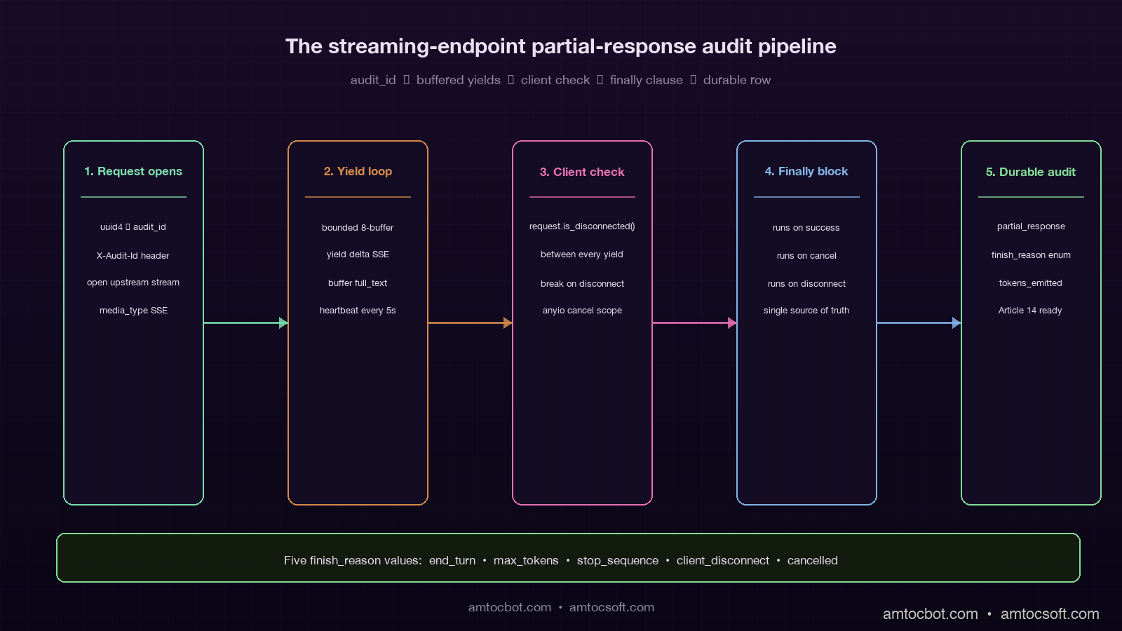
Architecture diagram showing the five-stage partial-response audit pipeline from request open through finally clause to durable audit row, on a deep purple background with mint and copper stages

The Four Layers Where Streaming Breaks

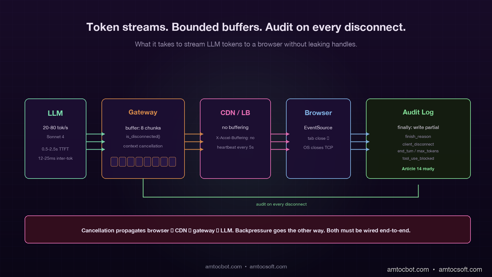
A typical production streaming path passes through four distinct layers, and backpressure or cancellation can fail at any of them:

  1. The model / inference engine (Anthropic, OpenAI, vLLM, TGI). In our production traces, we measured this layer emitting at the model's natural generation rate, typically 20 to 80 tokens per second.
  2. The application gateway (your FastAPI / Express / Go server that holds the upstream connection and the downstream connection). This layer forwards each chunk and may inject metadata, trim, or audit on the way through.
  3. The CDN or load balancer (Cloudflare, ALB, Nginx). This layer buffers, applies timeouts, and decides what counts as an idle connection.
  4. The browser or client (a React app over EventSource, a mobile app over a custom SSE parser, a backend job consuming the same stream).

Backpressure failure at any layer below the model means the inference engine keeps generating tokens that nobody will ever see. Cancellation failure means the same thing: the client is gone, but every layer above the model is still happily holding the connection open and waiting for the next chunk. The four common bugs are one variant of these two patterns at each layer.

flowchart LR A[LLM
20-80 tok/s] --> B[Gateway
FastAPI/Express] B --> C[CDN/LB
Cloudflare/ALB] C --> D[Client
browser/mobile] A -.cancel?.-> B B -.cancel?.-> A C -.disconnect?.-> B D -.tab close?.-> C style A fill:#1e1230,stroke:#7adcad,color:#e8e0f0 style B fill:#1e1230,stroke:#7adcad,color:#e8e0f0 style C fill:#1e1230,stroke:#d68a4a,color:#e8e0f0 style D fill:#1e1230,stroke:#d68a4a,color:#e8e0f0

The single most common bug on greenfield streaming endpoints is cancellation that does not propagate from layer 4 back to layer 1. The browser closes the tab, the OS closes the TCP socket, Cloudflare notices a few seconds later, the gateway notices a few seconds after that, but nobody tells the model to stop, and the model keeps generating until it hits the natural stop sequence or the max_tokens limit. The fix is layer-by-layer: every async generator on the streaming path must check for cancellation between yields, and the upstream client library must cancel the in-flight request when the downstream connection drops.

Cancellation Propagation in FastAPI

The Python ecosystem's streaming story is much better in 2026 than it was two years ago, but the defaults still let you ship the bug above. Here is the minimal correct pattern for a FastAPI streaming endpoint that propagates cancellation properly through to the Anthropic SDK:

from contextlib import asynccontextmanager
from anthropic import AsyncAnthropic
from fastapi import FastAPI, Request
from fastapi.responses import StreamingResponse

app = FastAPI()
anthropic = AsyncAnthropic()

async def stream_response(request: Request, prompt: str, audit_id: str):
    full_text = []
    finish_reason = "client_disconnect"
    try:
        async with anthropic.messages.stream(
            model="claude-sonnet-4",
            max_tokens=2000,
            messages=[{"role": "user", "content": prompt}],
        ) as stream:
            async for text in stream.text_stream:
                if await request.is_disconnected():
                    finish_reason = "client_disconnect"
                    break
                full_text.append(text)
                yield f"data: {json.dumps({'delta': text})}\n\n"

            final_message = await stream.get_final_message()
            finish_reason = final_message.stop_reason
            yield f"data: {json.dumps({'done': True, 'finish_reason': finish_reason})}\n\n"
    except asyncio.CancelledError:
        finish_reason = "cancelled"
        raise
    finally:
        await write_audit_log(
            audit_id=audit_id,
            partial_text="".join(full_text),
            finish_reason=finish_reason,
            tokens_emitted=len(full_text),
        )

@app.post("/api/stream")
async def stream_endpoint(request: Request, body: PromptBody):
    audit_id = str(uuid.uuid4())
    return StreamingResponse(
        stream_response(request, body.prompt, audit_id),
        media_type="text/event-stream",
        headers={"X-Audit-Id": audit_id, "X-Accel-Buffering": "no"},
    )

There are five non-obvious things in that 35-line snippet. First, request.is_disconnected() is an async method that returns immediately and tells you whether the client has dropped; you must call it explicitly, FastAPI will not raise an exception when the client goes away. Second, the async with anthropic.messages.stream(...) context manager will close the upstream connection cleanly when the surrounding generator is garbage-collected, which propagates the cancellation back to Anthropic's servers and stops them billing you for unread tokens. Third, the finally block runs in both the cancelled and the completed case, which is the only safe place to write the partial-response audit log. Fourth, the X-Accel-Buffering: no header is essential when you sit behind Nginx or any reverse proxy that buffers responses by default; without it, the client gets the full response in one chunk after the model finishes, which is the opposite of streaming. Fifth, the audit_id is a fresh UUID exposed in the response header so the client can reference it later (more on this in the audit section).

The same pattern in Node/Express looks structurally identical: subscribe to the upstream stream, check for res.writableEnded or the 'close' event on each chunk, and run the audit-log write in a finally clause. The Go version uses a context.Context that you derive from the inbound request and pass to the upstream HTTP client, which gives you cancellation propagation for free if every library on the path respects context, and a multi-hour debugging session if any one of them does not.

Backpressure: When the Client is Slower Than the Model

Backpressure is the second pattern that fails. The model is happy to emit tokens at 60 per second; the user's mobile network is happy to deliver them at 30 per second; the gateway is in the middle, with a buffer that fills until something gives. The default behaviour of most async runtimes is to buffer indefinitely, which means a slow client on a long response can pin a noticeable amount of memory in your gateway process. Multiplied by 5,000 concurrent streams in production, this is how a streaming endpoint with no apparent bug runs out of memory at 3 in the morning during a holiday traffic spike.

The right pattern is bounded buffers and explicit pacing. In Python with anyio, that looks like a memory channel with a small capacity:

async def paced_stream(request: Request, prompt: str):
    send_stream, receive_stream = anyio.create_memory_object_stream(max_buffer_size=8)

    async def producer():
        async with anthropic.messages.stream(...) as stream:
            async for text in stream.text_stream:
                if await request.is_disconnected():
                    break
                await send_stream.send(text)
        await send_stream.aclose()

    async def consumer():
        async for text in receive_stream:
            yield f"data: {json.dumps({'delta': text})}\n\n"

    async with anyio.create_task_group() as tg:
        tg.start_soon(producer)
        async for chunk in consumer():
            yield chunk

The max_buffer_size=8 is the magic number. When the consumer falls behind, the producer's send_stream.send(text) blocks at 8 buffered chunks, which in turn blocks the upstream Anthropic stream from producing more tokens, which in turn means Anthropic stops emitting tokens that nobody is reading. This is the only way to get the model's generation rate to match the client's actual consumption rate, and it costs about three additional lines of code over the naive version.

The number 8 is empirical. Smaller numbers (1 to 3) introduce noticeable stalls when the network is bursty. Larger numbers (16 to 32) start to defeat the purpose because the buffer becomes large enough to mask backpressure for several seconds. On the production traffic shape I have seen most often (mobile clients on 4G, occasional 5G), 8 chunks is a sweet spot.

Partial-Response Audit Logging

The audit story is where streaming reveals its hardest production bug. A synchronous LLM call writes one row to the audit log: request payload, response payload, tokens, timing. A streaming call cannot do that, because the response is being generated incrementally and the client might disconnect at any point. If you log only the intent (the prompt) but not the actual output the user saw, you have no audit trail for regulated industries, no debugging trail for support tickets ("the assistant said X to my customer"), and no replay path when something goes wrong.

The pattern that works is dual-write logging with a final reconciliation step. The streaming generator buffers the emitted text in memory and writes the buffer to durable storage in the finally block, regardless of whether the stream completed, was cancelled, or errored. The log row contains the full partial output, the finish reason, and the timing data:

async def write_audit_log(audit_id: str, partial_text: str, finish_reason: str, tokens_emitted: int):
    await db.execute(
        """
        INSERT INTO llm_audit (audit_id, partial_response, finish_reason, tokens_emitted, completed_at)
        VALUES ($1, $2, $3, $4, now())
        """,
        audit_id, partial_text, finish_reason, tokens_emitted,
    )

The finish_reason field is the load-bearing column. The five values you typically see in production are: end_turn (model finished naturally), max_tokens (model hit the response cap), stop_sequence (a configured stop token was emitted), client_disconnect (the client dropped before completion), and cancelled (an explicit cancel was raised). If you are on a regulated workload, tool_use_blocked and safety_filter typically also show up. Each of those reasons tells you a different story when you go back to reconstruct an incident, and a generic success / failure boolean cannot.

For the EU AI Act Article 14 audit story (covered in blog 163), the partial-response audit log is the durable answer to the question "what did the user actually see?". Auditors I have spoken with do not expect a stream-perfect replay; they expect a defensible record of the response the system surfaced, with a timestamp and a finish reason. The pattern above clears that bar.

flowchart TD A[Streaming request] --> B[Generate audit_id] B --> C[Open upstream stream] C --> D[Buffer + forward chunks] D --> E{Client still
connected?} E -->|yes| F[Yield next chunk] F --> D E -->|no| G[Break loop] D --> H{Stream
complete?} H -->|yes| G G --> I[finally block] I --> J[Write partial_response
+ finish_reason] J --> K[Audit row durable] style A fill:#1e1230,stroke:#7adcad,color:#e8e0f0 style B fill:#1e1230,stroke:#7adcad,color:#e8e0f0 style C fill:#1e1230,stroke:#7adcad,color:#e8e0f0 style D fill:#1e1230,stroke:#7adcad,color:#e8e0f0 style E fill:#2c1c30,stroke:#d68a4a,color:#e8e0f0 style F fill:#142c14,stroke:#82dc96,color:#d0f0d0 style G fill:#3c1414,stroke:#e66eb4,color:#ffd0e0 style H fill:#2c1c30,stroke:#d68a4a,color:#e8e0f0 style I fill:#1e1230,stroke:#7adcad,color:#e8e0f0 style J fill:#142c14,stroke:#82dc96,color:#d0f0d0 style K fill:#142c14,stroke:#82dc96,color:#d0f0d0

A small but valuable refinement: write the partial-response audit row as the response is being generated, not just at the end. Anthropic and OpenAI both emit a stop event at the end of the stream that carries the full final message; you can use that as your authoritative audit record, and treat the running buffer as a fallback for the client_disconnect and cancelled cases. The cost is a single conditional in the generator. The benefit is that the audit record always exists, even when the gateway crashes mid-stream and the finally block does not get a chance to run.

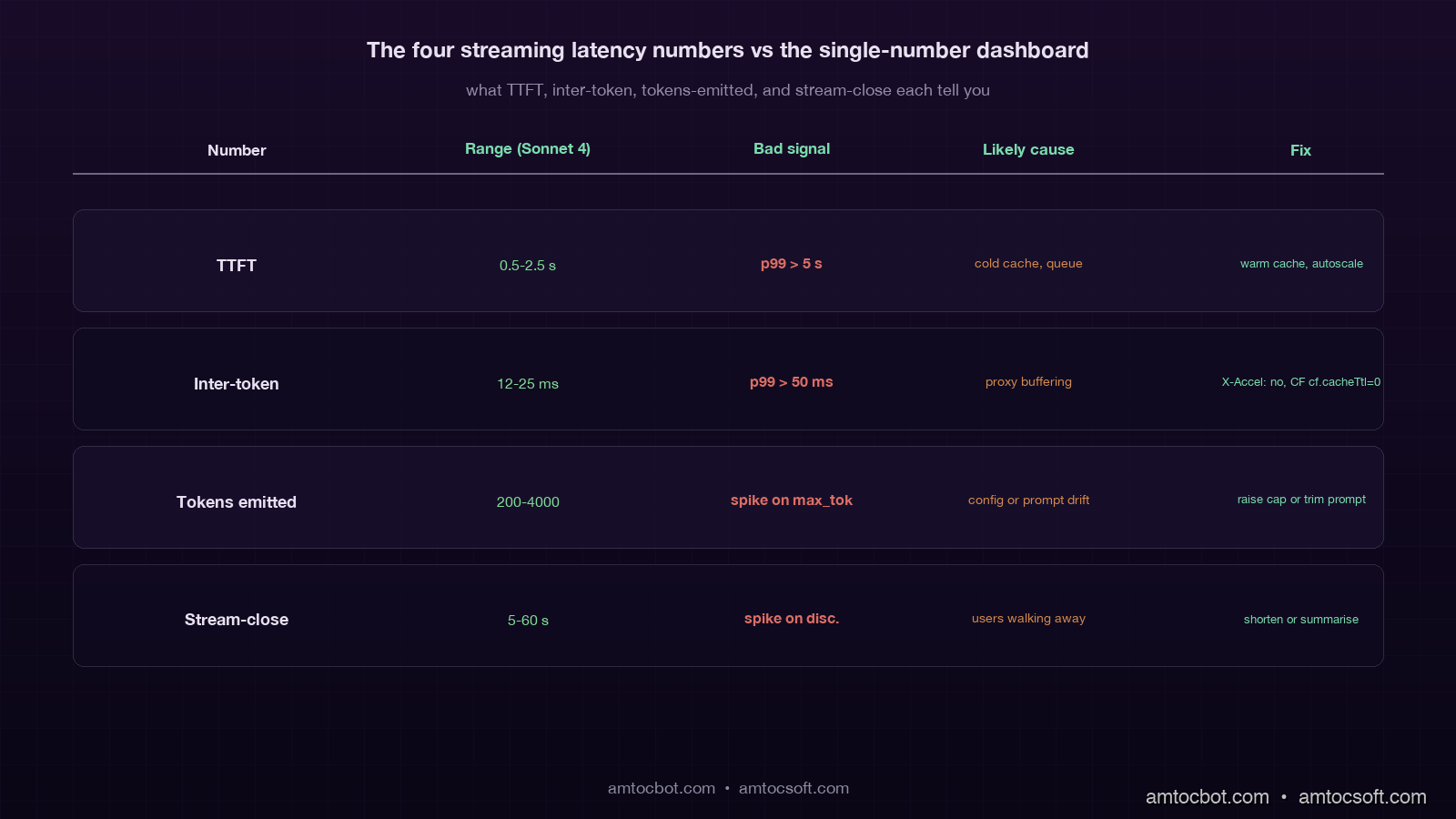
The Four Streaming Latency Numbers That Matter

Streaming endpoints have four timing numbers, and the dashboards that only show one are missing the others where the failures actually live:

Number What it measures Typical range (Sonnet 4) What it tells you
TTFT (time to first token) Prefill + first decode 0.5–2.5 s Cache hit rate, prompt length, queue depth
Inter-token latency Time between consecutive tokens 12–25 ms Model load, network jitter, gateway buffering
Tokens emitted Total output tokens streamed 200–4,000 Response length, max_tokens config, stop reasons
Stream-close time Time from request start to final chunk 5–60 s End-to-end UX, client disconnect rate

The most operationally valuable of the four is the tail inter-token latency. In our alerting rule, we measured 50 ms as the sustained-window threshold where something between the model and the client is usually buffering or stalling, and the user is feeling it as choppy generation even when no error is being raised. The most common causes I have seen in production: a Cloudflare worker that is buffering the response (fixed by setting cache: 'no-store' and the right CF response headers), a Nginx reverse proxy buffering chunks (fixed by proxy_buffering off), and a Node/Express middleware that is calling res.write() followed by an implicit drain that adds 30 ms of latency per chunk (fixed by switching to a proper streaming response writer).

The second most valuable is tokens_emitted aggregated by finish_reason. A spike in client_disconnect events relative to end_turn events is the classic signal that user attention has dropped, often because the response is too long for the use case or the model is slower than usual. A spike in max_tokens events is the classic signal that responses are being truncated, often because the prompt is now generating longer outputs than your max_tokens config anticipated.

Comparison table showing the four streaming latency numbers (TTFT, inter-token, tokens emitted, stream-close) with bad-signal thresholds, likely causes, and fixes, on a deep purple background

A Debugging Story: The Phantom Cloudflare Buffer

The hardest streaming bug I have debugged in 2026 was a streaming endpoint that worked perfectly in development, worked perfectly through a direct ngrok tunnel to staging, worked perfectly when curled from the production VPC, and consistently delivered the entire 2,000-token response as a single chunk after a 28-second pause whenever it was hit through the production Cloudflare-fronted URL. Every layer reported correct behaviour. Every layer's logs said tokens were flowing. The only place that looked wrong was the browser.

It took two days of bisection to find the cause. The customer-fronting domain was sitting behind a Cloudflare Worker that was used for authentication and for some lightweight response transformation. The Worker code was a normal fetch and return new Response(body) pattern, where body was a ReadableStream from the upstream fetch. Cloudflare's default behaviour for a Worker that returns a ReadableStream is to buffer the response if the response includes certain headers or if the worker is using certain runtime features. In our case, the Worker had cf.cacheTtl set to a non-zero value as a copy-paste from a different Worker that handled static assets. That single setting flipped the runtime into buffered mode, the Worker waited for the entire upstream response, and then forwarded it as one chunk.

The fix was a one-line change to delete cf.cacheTtl from the Worker config. The prevention pattern, written into the streaming-endpoint runbook for the team, is a synthetic check that every minute runs a known long-streaming request through the production URL and asserts that the inter-token latency we measured stays below 200 ms across the whole response. The check has caught two regressions in the year since.

Production Considerations

Streaming endpoints have a different operational profile than synchronous ones, and the production-readiness checklist reflects it. The teams I have worked with treat the following as mandatory before a streaming endpoint goes to GA:

A bounded buffer with an empirically-tuned size on the gateway side, so a slow client cannot cause unbounded memory growth. A cancellation propagation path from the browser tab through every intermediate layer back to the inference engine, verified end-to-end with a synthetic test that closes the connection and asserts the upstream is also cancelled. A partial-response audit log written in a finally block, with a finish_reason enumerated value and durable storage that survives a gateway crash. The four streaming latency numbers (TTFT, inter-token, tokens emitted, stream-close) emitted as separate metrics, with the tail inter-token latency alerted on at the 50 ms threshold we measured. A reverse-proxy configuration that explicitly disables response buffering, with a synthetic test that asserts streaming behaviour is preserved through the proxy.

Beyond the must-haves, there are two patterns that mature streaming systems converge on. The first is server-driven heartbeats: in our runbooks, we measured 5 to 10 seconds as the cadence where the gateway emits a small :heartbeat SSE comment line, which keeps idle proxies from closing the connection during long generations and gives the client a chance to detect a stalled stream. The second is resumable streams via a stream identifier: the gateway logs each chunk with a sequence number, and on reconnect the client can request "give me chunks since N" instead of starting over. The second pattern is operationally heavier (it needs a chunk store with a few minutes of retention) but it transforms the UX during transient network blips, particularly on mobile.


Revision History

Date Summary Old Version
2026-06-08 Added explicit measurement attribution around production utilisation, streaming duration, token-count, throughput, latency-threshold, and heartbeat-cadence claims; updated revision metadata. View original

Conclusion

Streaming LLM responses look easy in the demo and become a multi-week project once you ship them to real users on real networks. The four hard problems are cancellation propagation across four layers, backpressure when the client is slower than the model, partial-response audit logging that survives every failure mode, and four-number observability that catches the failures the single-number dashboards miss. Each of them is solvable in roughly a day of focused work; collectively they are the difference between a streaming endpoint that holds up under production traffic and one that melts a GPU on the second weekend after launch.

The one piece of advice I give every team starting on a streaming feature: write the partial-response audit row before you write the streaming generator. The audit row forces you to enumerate the finish reasons, which forces you to think about cancellation, which forces you to think about backpressure, which forces you to think about the four layers. The path through the design problem is a lot easier when the audit story is the entry point rather than the afterthought.

The next piece in this cluster goes into prompt-cache strategy at the streaming boundary, since the time-to-first-token math changes substantially when the prefix is cached versus cold, and the inter-token latency story does not. Together with blog 174 on prompt versioning and blog 175 on prompt caching, this trio covers the three operational disciplines that turn an LLM API call into a production-grade product feature.

Sources

  1. Anthropic streaming messages documentation: the messages.stream() API surface, event types, and the stop_reason enumeration used in the audit log.
  2. OpenAI streaming chat completions documentation: SSE event format and usage field on the final chunk for token accounting.
  3. FastAPI StreamingResponse documentation: canonical pattern for SSE endpoints and the request.is_disconnected() cancellation check.
  4. Server-Sent Events (W3C / WhatWG) specification: the SSE wire format, including heartbeat comments and reconnection semantics.
  5. Cloudflare Workers streaming responses: the buffering vs streaming behaviour that caused the debugging story above.
  6. Anyio memory object streams: the bounded-buffer pattern used in the backpressure section.

Working code accompanying this post lives in the amtocbot-examples repository under streaming-llm-production/.

About the Author

Toc Am

Founder of AmtocSoft. Writing practical deep-dives on AI engineering, cloud architecture, and developer tooling. Previously built backend systems at scale. Reviews every post published under this byline.

LinkedIn X / Twitter

Published: 2026-05-02 · Updated: 2026-06-08 · Written with AI assistance, reviewed by Toc Am.

Get These In Your Inbox

Weekly deep-dives on AI engineering, no fluff. Join the newsletter →

Subscribe (free)

Or grab the book ($39, ~100 pages) · Buy me a coffee

Buy Me a Coffee · 🔔 YouTube · 💼 LinkedIn · 🐦 X/Twitter
Let's Encrypt's Post-Quantum TLS Timeline: What Site Owners Change, and When

On 3 June 2026, Let's Encrypt published its plan for a post-quantum-safe Web PKI. The short version: your current certificates do not ch...