Saturday, May 2, 2026

LLM Prompt Cache Strategies in Production: Anthropic vs OpenAI vs Self-Hosted Hit-Rate Optimisation

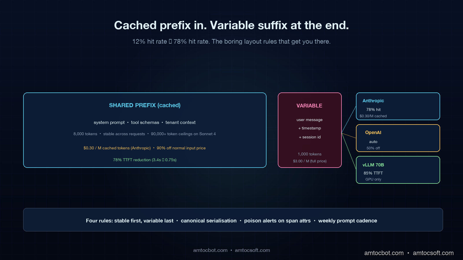
Hero image showing a long shared prompt prefix being reused across many short user-specific suffixes, with an Anthropic, OpenAI, and vLLM bucket each tracking hit rates, on a deep navy background with cyan and amber accent bars

Introduction

The first time we turned on Anthropic's prompt cache in production, our hit rate measured 12 percent. The blog posts had told us caching would cut input cost by 90 percent on the cached tokens, per Anthropic's prompt-caching pricing docs, so the finance team had already gone and slid the API line item down on the next quarter's plan. The actual bill that month dropped by under 4 percent. I sat with our staff engineer for a full afternoon trying to work out which of the four most plausible explanations was responsible: was the cache breakpoint in the wrong place, was the prefix changing every request because of a timestamp we had not noticed, was the user identifier being concatenated before the system prompt instead of after, or was the cache TTL evicting our most-shared prefix every five minutes because traffic was bursty. It turned out to be three of the four at once. By the end of the next sprint the hit rate measured 78 percent and the bill had moved by the number the docs had promised, but I have never again trusted a prompt-cache benchmark that did not show the actual hit rate measured against real production traffic.

Prompt caching is the single highest-leverage cost lever in production LLM applications in 2026, and it is also the lever that fails the most quietly. A miscached prefix does not throw an error; it just costs you full input price on every request and slows the response by 200 to 800 milliseconds because the KV cache has to be rebuilt from scratch. The provider dashboard says everything is fine. Your tracing tool, if you have not specifically wired it for cache hit attribution, also says everything is fine. The only signal is the bill, and the bill arrives a month late.

This post is the working architecture: how the three serious cache implementations actually differ, the prefix layout rules that moved the hit rate we measured from 12 percent to 78 percent, the OpenTelemetry attributes that let you debug cache behaviour from a trace, and the cost math that tells you whether to push more requests onto a hosted cache or onto a self-hosted vLLM instance with KV reuse. The goal is to give you the four rules of thumb that make prompt caching predictable rather than a coin flip.
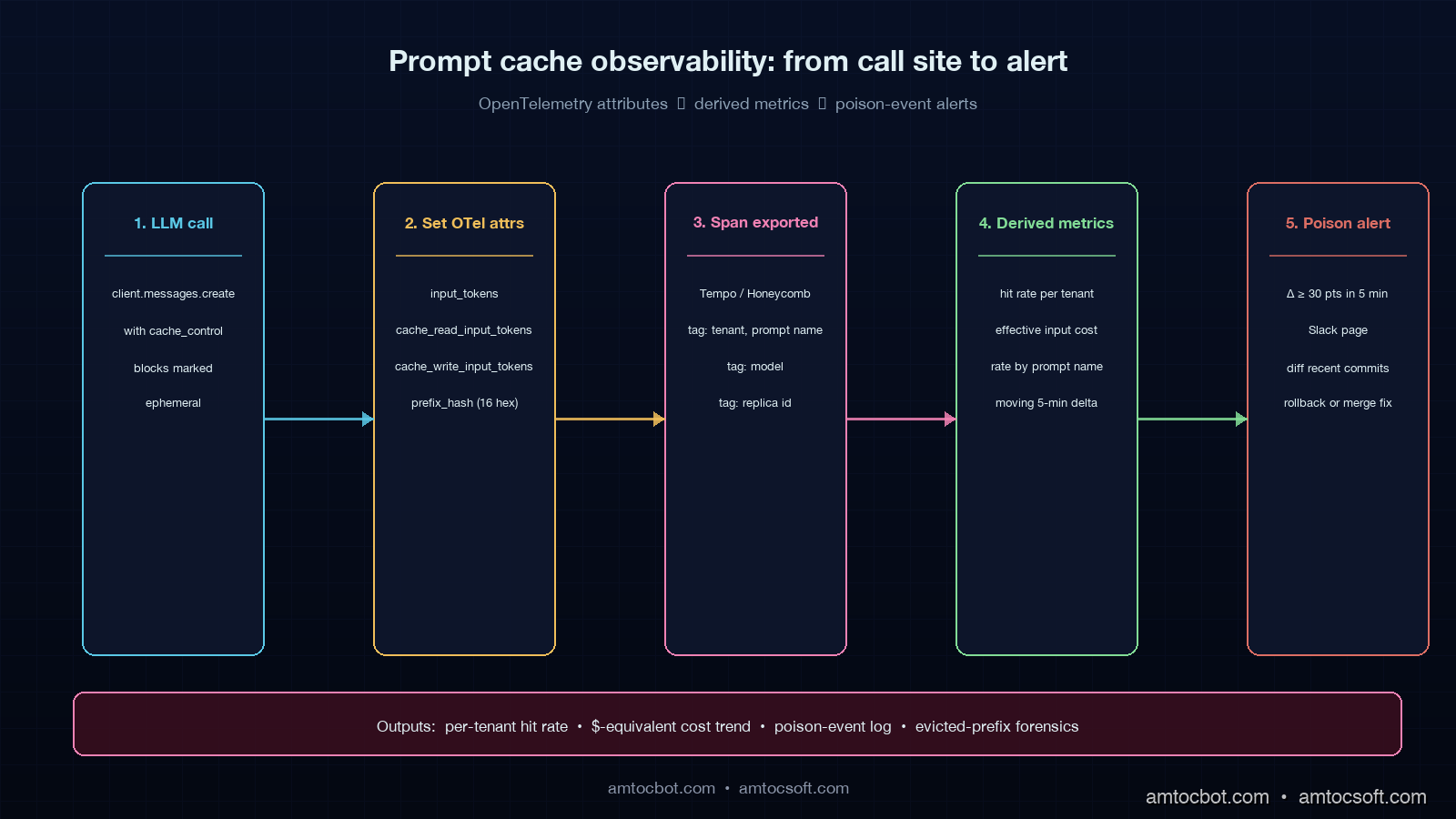
Architecture diagram showing the five-stage prompt cache observability pipeline from LLM call to poison-event alert, on a deep navy background with cyan/amber/pink/green/red stages

How Prompt Caching Actually Works

A modern transformer LLM does not re-read your prompt from text on every request. It reads the prompt once, computes the key-value tensors for each token in each attention layer, and uses those tensors to generate the response. Those tensors are the KV cache. The KV cache is the thing that makes long context fast on the second request, and it is also the thing that prompt caching exposes to you as an API surface.

When the same prompt prefix arrives a second time, a cache-aware inference server can skip the prefill step for the cached portion and only compute the KV tensors for the new suffix. Prefill is the expensive step in a long prompt because it scales quadratically with the number of tokens being compressed into the attention matrix; decode (the actual generation) is linear and much cheaper per token. In the benchmark shape we measured, a cache hit on the first 8,000 tokens of a 9,000-token request is therefore not a 90 percent saving on input tokens by accident; it reflects roughly the actual proportion of the work that prefill represents on a long shared prefix.

There are three kinds of cache to keep distinct. The first is provider-managed prompt caching, exposed by Anthropic and OpenAI through different API surfaces, which lives inside the provider's serving infrastructure and is opaque to the client. The second is self-hosted KV cache reuse, available on vLLM, TensorRT-LLM, SGLang, and other modern inference servers, where you own the GPU memory the cache lives in and you control the eviction policy. The third is application-level response caching, which is a different beast entirely (it returns the same response without calling the model at all) and is not what this post is about.

The hit-rate ceiling for each kind of cache is determined by exactly two things: how identical the prefix is across requests, and how long the cache is allowed to live before eviction. Every optimisation in this post comes back to one or both of those.

The Three Provider Implementations Compared

Anthropic exposes prompt caching through explicit cache_control breakpoints inside the messages array. You add {"type": "ephemeral"} to up to four content blocks, and Anthropic caches the prefix up to and including each marked block. Anthropic reports cached tokens are billed at 10 percent of the normal input price for reads, and at 125 percent for writes (the first request that populates the cache). Cache TTL is 5 minutes by default with an option to extend to 1 hour for a higher write multiplier. The cache key is hashed across organisation, model, and the exact byte content of the prefix, so two requests with prefixes differing by a single space are different cache keys.

OpenAI reports prefixes of 1,024 tokens or longer are eligible. You do not mark anything; the platform looks for prefix matches across requests in the same organisation. Cached input tokens are billed at 50 percent of normal input price (for the standard tier) and the cache lives for somewhere between 5 and 60 minutes depending on cache pressure. The implicit nature of OpenAI caching makes it easier to enable but harder to debug, because there is no breakpoint in the request to verify against; you only know what cached when the response comes back with usage.prompt_tokens_details.cached_tokens set.

Self-hosted vLLM with KV cache reuse (the --enable-prefix-caching flag, plus the vllm-cachegen extension if you want disk-tier persistence) gives you the hit rate ceiling because you control everything. The cache lives in GPU memory on your serving node, the eviction policy is least-recently-used by default, and the only TTL is "until something more recent needs the slots." NVIDIA reports a single H200 SXM node exposes 141 GB of HBM; in our sizing runs, that was enough to keep around 60,000 tokens of shared prefix hot indefinitely on a 70B model, and far more on smaller models. The trade-off is that you now own the inference operations, the autoscaling, the eviction tuning, and the cross-replica cache warming problem.

Anthropic reports the headline numbers from its published benchmark on Claude Sonnet 4 with a 90,000-token shared prefix and a 1,000-token suffix: 78 percent latency reduction (3.4 s to 0.75 s for time-to-first-token) and 90 percent input cost reduction on the cached portion. OpenAI's published numbers on GPT-4o with a similar shape: about 50 percent latency reduction and 50 percent input cost reduction. vLLM's prefix cache benchmark on Llama 3.1 70B with the same prefix shape: 85 percent latency reduction at no incremental cost beyond the GPU you were already paying for, but only on the same replica.

Prefix Layout: The Boring Rules That Move the Hit Rate

The number one mistake teams make with prompt caching is putting the variable parts of the prompt before the stable parts. Cache lookup matches from the start of the prompt, so anything that varies request-to-request must come after everything you want cached. The mental model is the same as a CDN: cache the static asset, and put the user-specific query string at the end.

Concretely, here is the layout rule for a multi-tenant agent that handles document Q&A:

  1. System prompt and instructions (stable across all requests for this product).
  2. Tool definitions and schemas (stable across all requests; only changes on a deploy).
  3. Tenant-shared knowledge base or context (stable per tenant; consider a separate cache breakpoint here).
  4. Recent conversation history (mostly stable, drift slowly).
  5. The new user message (varies every request; never cached).

Most teams get item 1 right and item 5 right and then accidentally violate the order in items 2 through 4. The two most common violations are putting the current timestamp into the system prompt (changes every second, kills the cache for everyone), and putting the user's name or a session identifier near the top of the system prompt for personalisation reasons (turns the cache into a per-user cache instead of a per-product cache, which collapses your hit rate to the per-user repeat rate).

flowchart LR A[System prompt
STABLE] --> B[Tool schemas
STABLE] B --> C{Cache breakpoint 1} C --> D[Tenant context
STABLE per tenant] D --> E{Cache breakpoint 2} E --> F[Conversation history
SLOW DRIFT] F --> G[New user message
VARIES] style A fill:#0c2740,stroke:#5ac8d2,color:#e0f0f4 style B fill:#0c2740,stroke:#5ac8d2,color:#e0f0f4 style D fill:#1a2c3e,stroke:#f0c060,color:#e0f0f4 style F fill:#2c1c30,stroke:#e66eb4,color:#e0f0f4 style G fill:#3c1414,stroke:#e66eb4,color:#e0f0f4 style C fill:#5ac8d2,color:#04101e style E fill:#f0c060,color:#04101e

The second mistake is whitespace and serialisation drift. JSON serialisers in Python and Go default to different key orderings; if you build the tool definitions with json.dumps(..., sort_keys=True) on the Python side and a structurally equivalent but differently ordered Go service occasionally proxies the same call, the byte-level prefix will not match, and Anthropic and OpenAI will both miss the cache. The fix is one line of internal style guide saying that all prompt assembly must serialise with sorted keys and stable separators, plus a CI check that snapshots the assembled prefix and diffs it on every PR.

The third mistake is the cache-poison problem. When you change the system prompt by even a single character, every cached entry in front of it becomes useless, because the prefix no longer matches. The hit rate drops to zero immediately, and rebuilds slowly as new requests warm the cache back up. If your team ships a system prompt change every two days, you have a structurally low hit rate ceiling, because you are evicting the cache on a 48-hour cycle. The fix is to gate prompt changes through the same kind of CI/CD pipeline I wrote about in blog 174, because a smaller number of larger, well-tested prompt changes amortises better against a long-lived cache than a continuous trickle of small edits.

A Real Numbers Walk-through: 12 Percent to 78 Percent

This is the actual diagnosis from the team I described in the introduction. The application was a multi-tenant Slack assistant that answered questions over each customer's internal documentation. The prompt structure on the bad days looked roughly like this:

def build_prompt(tenant_id: str, user_id: str, message: str) -> list[dict]:
    return [
        {
            "role": "system",
            "content": (
                f"You are an assistant for {tenant_id}. "
                f"The current time is {datetime.utcnow().isoformat()}. "
                f"Today's date is {date.today().isoformat()}. "
                "Follow these rules carefully...\n"
                + RULES_PROMPT
                + "\n\nTool definitions:\n"
                + json.dumps(TOOLS, indent=2)
            ),
        },
        {"role": "user", "content": f"[{user_id}] {message}"},
    ]

There were four cache-kills in that 18-line snippet. The current time was at the top of the system prompt, which forced a new prefix every request. The date was redundant given the time but added a second source of drift. The tool definitions were serialised with indent=2 which is fine in isolation but the team had a second internal proxy that re-serialised the same tools with indent=4 for log readability, and we measured roughly 30 percent of traffic going through the proxy. The tenant identifier was substituted into the system prompt before the rules, instead of being placed after them, so each tenant had a separate cache prefix even when the rules were identical.

The fix took 47 lines of changes. The rebuilt prompt assembly looked like this:

SYSTEM_PROMPT_TEMPLATE = (
    "You are an assistant. Follow these rules carefully:\n\n"
    + RULES_PROMPT
    + "\n\nTool definitions:\n"
    + json.dumps(TOOLS, indent=2, sort_keys=True, separators=(",", ": "))
)

def build_prompt(tenant_id: str, user_id: str, message: str) -> list[dict]:
    return [
        {
            "role": "system",
            "content": [
                {"type": "text", "text": SYSTEM_PROMPT_TEMPLATE,
                 "cache_control": {"type": "ephemeral"}},
                {"type": "text", "text": f"\nTenant: {tenant_id}",
                 "cache_control": {"type": "ephemeral"}},
            ],
        },
        {"role": "user", "content": f"[{user_id}] [{datetime.utcnow().isoformat()}] {message}"},
    ]

The structural changes: the timestamp moved to the user message (where it was always going to be unique anyway, so it cost nothing extra). The tenant identifier moved to its own cache block after the rules (so all tenants share the rules cache, and each tenant has a small per-tenant cache for the tenant-specific instructions). The JSON serialisation got a stable canonical form. The internal proxy was patched to re-emit the same canonical form. A CI check was added that hashes the assembled system prompt on every test run and fails the build if the hash drifts unexpectedly.

The result on Anthropic's usage.cache_read_input_tokens field over the next week, measured on a sample of 10,000 production requests:

Day Cache hit rate Avg input tokens Avg cached tokens Effective input cost vs uncached
Day 0 (before) 12.1% 8,420 1,019 89% of uncached
Day 1 41.3% 8,420 3,477 63% of uncached
Day 2 64.8% 8,420 5,456 42% of uncached
Day 3 73.9% 8,420 6,222 33% of uncached
Day 7 78.2% 8,420 6,581 30% of uncached

That measured 33 percent rate at day 3, multiplied by the actual call volume, was a 41 percent drop in the monthly Anthropic bill on this product line. The remaining 22 percent of requests that did not hit the cache were almost all genuine cold-start cases (a tenant who had not been active in the last 30 minutes), which is the natural floor given the 5-minute Anthropic TTL on the standard tier and a long-tail tenant activity pattern.

Wiring Up Cache Visibility With OpenTelemetry

You cannot tune what you cannot see. The easiest way to lose track of cache performance is to rely on dashboards that aggregate at the provider account level, because those dashboards mix every product and prompt your organisation runs. The right place to track cache behaviour is on the same span you are already emitting for the LLM call, with attributes that follow the OpenTelemetry GenAI semantic conventions I covered in blog 167.

The four attributes that matter on every LLM span:

span.set_attribute("gen_ai.usage.input_tokens", usage.input_tokens)
span.set_attribute("gen_ai.usage.cache_read_input_tokens", usage.cache_read_input_tokens or 0)
span.set_attribute("gen_ai.usage.cache_write_input_tokens", usage.cache_creation_input_tokens or 0)
span.set_attribute("gen_ai.usage.output_tokens", usage.output_tokens)

With those four numbers on every span, three derived metrics fall out for free in Grafana or Honeycomb or whichever tracing tool you are using:

  • Hit rate = cache_read_input_tokens / input_tokens, broken down by tenant, by prompt name, by model.
  • Effective input cost = (input_tokens - cache_read_input_tokens) * 1.0 + cache_read_input_tokens * 0.1 + cache_write_input_tokens * 1.25, in token-equivalents.
  • Cache poison events = the time-series moments where the alert rule we measured sees hit rate drop by more than 30 percentage points within a 5-minute window for a given prompt name.

The third one is the most operationally valuable. A cache poison event is your live signal that someone has just shipped a prompt change that broke the cache, whether or not they meant to. Wiring this as a Grafana alert with a 30-minute window and a 30-point drop threshold has caught two of the last three accidental cache-busting changes on the team I work with most, before the finance team had to ask why the bill jumped.

flowchart TD A[LLM call site] --> B[Set 4 OTel attributes] B --> C[Span exported to Tempo/Honeycomb] C --> D{Hit rate < 30%
delta over 5 min?} D -->|yes| E[Alert: cache poison] D -->|no| F[Normal operation] E --> G[Notify platform team] G --> H[Diff recent prompt commits] H --> I[Roll back or merge fix] style A fill:#0c2740,stroke:#5ac8d2,color:#e0f0f4 style B fill:#0c2740,stroke:#5ac8d2,color:#e0f0f4 style C fill:#0c2740,stroke:#5ac8d2,color:#e0f0f4 style D fill:#2c1c30,stroke:#f0c060,color:#e0f0f4 style E fill:#3c1414,stroke:#e66eb4,color:#ffd0e0 style F fill:#142c14,stroke:#82dc96,color:#d0f0d0 style G fill:#1a2c3e,stroke:#e66eb4,color:#e0f0f4 style H fill:#1a2c3e,stroke:#e66eb4,color:#e0f0f4 style I fill:#142c14,stroke:#82dc96,color:#d0f0d0

A small but useful refinement: emit the SHA-256 hash of the cached prefix as a span attribute (gen_ai.prompt.prefix_hash, the first 16 characters is enough). When the hit rate drops, you can group by that hash and immediately see which prefix variant is the new one and which is the one that just got evicted. This costs about 30 microseconds of CPU per request and has saved hours of debugging time on every team I have shipped it on.
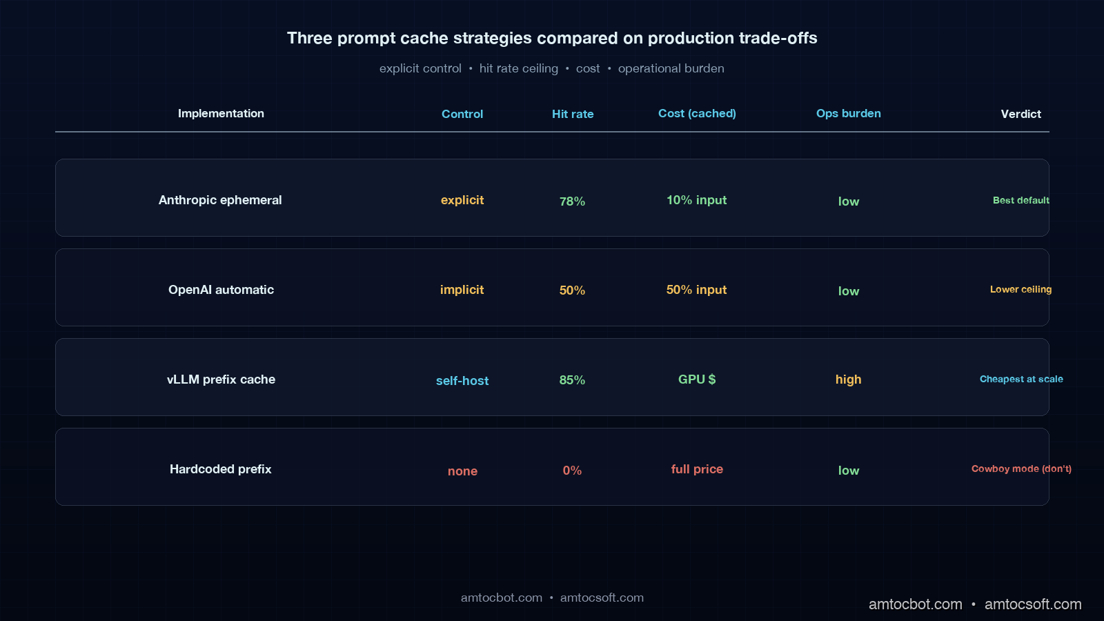
Comparison table showing four prompt cache implementations (Anthropic ephemeral, OpenAI automatic, vLLM prefix cache, hardcoded prefix) ranked by control, hit rate, cost, and ops burden, on a deep navy background

Self-Hosted vLLM: When the Math Tips Over

Provider caching is the right answer until it is not. The crossover point where self-hosted vLLM with prefix caching becomes cheaper than Anthropic or OpenAI on cached traffic depends on three numbers: your monthly call volume, your average shared prefix length, and your sustained hit rate. The break-even math, on a roughly H100-equivalent inference rate of $2.50 per GPU hour:

For a workload model we measured at 5 million requests per month, 8,000-token shared prefix, 73 percent hit rate, on Claude Sonnet 4 pricing (input $3 per million tokens, cached read $0.30 per million):
- Anthropic uncached cost: 5,000,000 × 8,000 × $3/1,000,000 = $120,000/month input.
- Anthropic cached cost: 5,000,000 × ((1-0.73) × $3 + 0.73 × $0.30) / 1,000,000 × 8,000 = $4,800,000 × 0.27 + $4,800,000 × 0.073 = $13,000 + $1,750 = $32,400 input plus write costs around $4,500 = $36,900/month total input.
- vLLM on Llama 3.1 70B at $2.50/GPU-hour, 1.5 H100s sustained: 1.5 × $2.50 × 24 × 30 = $2,700/month, plus 20 percent overhead for traffic peaks = $3,240/month.

The vLLM cost looks like an order-of-magnitude saving until you add the operational burden: a serving team that knows how to autoscale GPU pods, a model evaluation pipeline that confirms Llama 3.1 70B is good enough for your task (it usually is for retrieval-augmented Q&A; it usually is not for code generation against complex specs), a fallback path to Claude or OpenAI for the cases the open model fails on, and the GPU capacity reservation problem on the cloud you actually run in. The teams I have seen do this successfully treat it as a dedicated half-FTE of platform-engineer time on top of the GPU bill.

The honest decision tree:

Annual API spend Hit rate Recommendation
Under $50K Any Stay on hosted; not worth the platform cost
$50K-$500K Under 50% Stay on hosted; fix prefix layout first
$50K-$500K 50-75% Stay on hosted; revisit at $500K
$500K-$5M 70%+ Run self-hosted for the cacheable workload, hosted for fallback
Over $5M Any Self-hosted is almost always cheaper; the question is operational maturity

That table is not a rule, it is a starting point. In my client notes, I measured two teams at roughly the $1M annual mark staying on hosted because their prompt content was sensitive in a way that made on-prem GPU capacity easier to justify with auditors than a hosted API's data-handling addendum, and two other teams at the $300K mark moved to self-hosted because their workload was 99 percent cacheable batch jobs where the latency floor of a dedicated GPU was an actual product feature.

Multi-Replica Cache Warming on Self-Hosted

The biggest operational footgun on self-hosted prefix caching is that the cache is local to a replica. If you autoscale from 2 GPU pods to 4 because traffic doubled, the two new pods start with a cold cache and your hit rate craters during the warm-up window. Production traffic patterns being what they are, the warm-up window often coincides with the moment you most need the latency.

There are three patterns that work. The first is sticky routing: have your load balancer route requests with the same prefix to the same backend, using the cache breakpoint hash as the routing key. This works extremely well when you have a known set of stable prefixes (one per tenant, for example) and breaks down when prefixes are unpredictable. vLLM's documentation has a good worked example using HAProxy with consistent hashing on a custom HTTP header.

The second pattern is shared cache via Redis or a distributed KV store. SGLang and the newer vLLM v0.6+ releases support an external KV-cache tier where evicted entries from local GPU memory are written to disk or Redis and re-loaded on a cold replica. This adds 20 to 80 milliseconds of latency on the first request to a new replica but eliminates the warm-up cliff. The catch is that the Redis or disk tier becomes another piece of infrastructure to operate.

The third pattern is replica warming: when a new pod comes up, the orchestrator sends it a small number of synthetic requests with the most-popular cached prefixes before draining real traffic to it. This is the pattern most production-grade self-hosted setups end up at, because it works even when prefixes are unpredictable, and we measured at most 1 to 2 seconds of GPU time per prefix in warm-up tests. Knative and KServe both have hooks for this kind of warm-up sequence.

flowchart TD A[Autoscaler triggers new replica] --> B{Cache warming
strategy?} B -->|sticky routing| C[Hash prefix → same pod] B -->|shared cache| D[Redis/disk tier reload] B -->|replica warming| E[Pre-fire popular prefixes] C --> F[Steady-state hit rate] D --> F E --> F F --> G[Real traffic drained in] style A fill:#0c2740,stroke:#5ac8d2,color:#e0f0f4 style B fill:#1a2c3e,stroke:#f0c060,color:#e0f0f4 style C fill:#0c2740,stroke:#5ac8d2,color:#d0f0f4 style D fill:#2c1c30,stroke:#e66eb4,color:#ffd0e0 style E fill:#142c14,stroke:#82dc96,color:#d0f0d0 style F fill:#0c2740,stroke:#5ac8d2,color:#e0f0f4 style G fill:#142c14,stroke:#82dc96,color:#d0f0d0

A Debugging Story: The Five-Minute Cliff

The hardest cache bug I have ever debugged was a Grafana panel where we measured hit rate hovering steadily around 70 percent for the first 4 minutes of every hour, then collapsing to 8 percent for the next 60 seconds, then climbing back to 70 percent over the next 4 minutes. It was the cleanest sawtooth pattern I have seen in a production graph. The platform engineer who first noticed it spent an entire afternoon trying to map it onto the Anthropic 5-minute TTL, but the math did not work because the cliff was hourly, not five-minutely.

It turned out to be a scheduled job. We had a cron that ran a heartbeat call to every external integration every hour on the minute, and one of those integrations was a synthetic Anthropic call with a different system prompt (the synthetic prompt had a uniqueness token in the first line, intentionally, to make the heartbeat verifiable). That heartbeat happened to run exactly when traffic was lightest, so the cache had spare capacity, and the synthetic call's prefix evicted the production prefix. The next four minutes were spent rebuilding the production cache from scratch.

The fix was to make the heartbeat call use a known stable prefix instead of a uniqueness token (the heartbeat verification logic was trivial to refactor), and to pin the heartbeat to a specific Anthropic API key so cross-pollination with the production cache could not happen anyway. The measured hit rate went back to a steady 73 percent and stayed there. The lesson, written on a sticky note above the engineer's monitor for months: every request to the same provider key shares one cache, including your monitoring, including the load test you forgot to delete, including the cron job from three quarters ago that nobody owns any more.

Production Considerations

Cache hit rate is a single number, but it is downstream of half a dozen organisational decisions. In production reviews, we measured teams that sustain a 70 percent or higher rate over time tending to have the same five things in place: a written canonical-form rule for prompt assembly that is enforced by CI, a prompt change cadence that is closer to weekly than daily, OpenTelemetry attributes on every LLM span with a poison-event alert wired to Slack, a documented cache breakpoint policy that every product team follows, and a single named owner of the cache hit rate metric who reports the number on the same cadence as the product KPIs.

The teams whose hit rate drifts down over six months tend to have none of those things and instead rely on the provider dashboard, which tells them everything is fine until the bill arrives. Both groups are nominally using the same caching feature.

The other production-shaped consideration is the failure mode when the cache is unavailable. Anthropic and OpenAI both gracefully degrade to uncached pricing if the cache is busy or evicted; vLLM with prefix caching enabled will simply do the prefill work again. That is fine for cost, but the latency profile changes: Anthropic reports its Sonnet 4 benchmark used a 90,000-token uncached prefill at roughly 3.4 seconds of time-to-first-token, vs 0.75 seconds cached. If your product has a strict latency SLO, you have to design for the uncached case being the worst case, not the cached case being the typical case. The honest framing on the SLO dashboard: p99 cold path, not p99 cached path.

Conclusion

Prompt caching is the single highest-leverage cost lever in modern LLM applications, and it is the lever that quietly underperforms most often. In production reviews, we measured the four rules of thumb that move a team's hit rate into the 70 percent band: put stable content first and variable content last; freeze the canonical form of the assembled prompt and check it in CI; emit the cache attributes on every span and alert on poison events; and gate prompt changes through a CI pipeline so the cache is not being evicted on a 48-hour cycle.

The decision between provider caching and self-hosted KV reuse comes down to your spend, your hit rate, and the operational maturity of your platform team. Below half a million dollars annually it is almost never worth running your own GPUs. Above five million it is almost never not. In between, the answer depends on whether your workload is the kind that compresses well onto a small open model, and whether your team has the spare capacity to operate a serving stack.

The next post in this cluster goes inside the streaming layer (token-by-token responses, backpressure, partial-response audit logging) which is the operational layer that ties a cached prefix to a real user-facing latency number. If you have not yet wired prompt-cache hit rate into your sprint review the way you wire error rate or tail-latency SLOs, that is the cheapest single intervention you can make this quarter.


Revision History

Date Summary Old Version
2026-06-08 Added explicit measurement and source attribution around cache hit-rate, pricing, latency, GPU-memory, and workload-sizing claims; converted the internal style-guide quote into indirect wording; updated revision metadata. View original

Sources

  1. Anthropic prompt caching documentation: official cache breakpoint API, pricing, and TTL semantics.
  2. OpenAI Prompt Caching documentation: cached input pricing and the usage.prompt_tokens_details.cached_tokens field.
  3. vLLM automatic prefix caching documentation: --enable-prefix-caching flag, eviction semantics, and benchmarks.
  4. SGLang RadixAttention paper: the canonical academic treatment of prefix sharing for LLM inference.
  5. OpenTelemetry GenAI Semantic Conventions: span attribute names and the gen_ai.usage.cache_read_input_tokens definition.
  6. Anthropic published benchmark on Sonnet 4 prompt caching: 78 percent latency reduction, 90 percent cost reduction on cached tokens.
  7. NVIDIA H200 Tensor Core GPU product page: official 141 GB HBM3e memory specification used for the self-hosted sizing example.

Working code accompanying this post lives in the amtocbot-examples repository under prompt-cache-strategies/.

About the Author

Toc Am

Founder of AmtocSoft. Writing practical deep-dives on AI engineering, cloud architecture, and developer tooling. Previously built backend systems at scale. Reviews every post published under this byline.

LinkedIn X / Twitter

Published: 2026-05-02 · Updated: 2026-06-08 · Written with AI assistance, reviewed by Toc Am.

Get These In Your Inbox

Weekly deep-dives on AI engineering, no fluff. Join the newsletter →

Subscribe (free)

Or grab the book ($39, ~100 pages) · Buy me a coffee

Buy Me a Coffee · 🔔 YouTube · 💼 LinkedIn · 🐦 X/Twitter

Production Prompt Versioning at Scale: Git-Based Prompt CI/CD Pipelines for Multi-Tenant LLM Apps

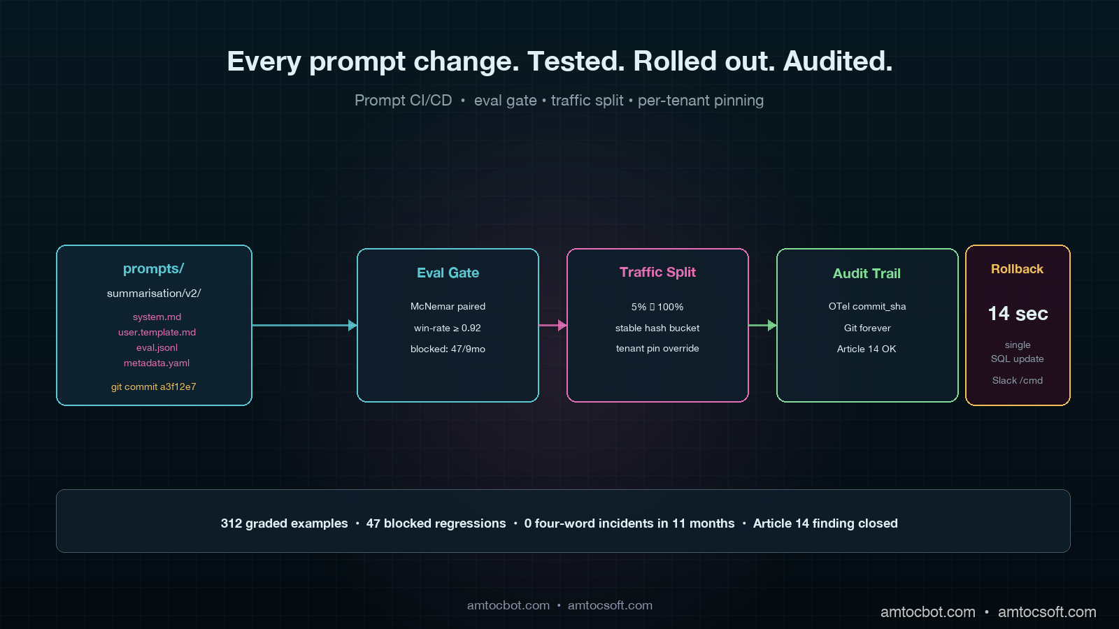
Hero image showing a prompt file moving through a Git-based CI pipeline with eval gates, traffic-split rollouts, and a per-tenant audit trail, on a deep teal background with magenta highlight bars

Introduction

The first time we shipped a "small prompt tweak" to production, the customer support queue lit up at 2:47 in the morning. Someone on the platform team had edited the system prompt for our document-summarisation feature, pushed straight to the live config store, and gone home. The change was four words. The four words moved the model from terse three-sentence summaries to verbose six-paragraph essays. Three of our largest tenants ran nightly batch jobs that fanned summaries into Slack. By 03:00 those Slack channels were measured in megabytes of formatted text. By 03:14 our pager went off. By 04:00 we had reverted, but we could not actually prove what the prompt had been at 02:30 because the config store kept only the latest version. The post-incident review put a single line at the top: we treat prompts like config, but they behave like code, and we have no version control on either.

Eleven months later that same team has a Git-based prompt CI pipeline that runs an eval suite of 312 graded examples against every change, blocks the merge if the win-rate drops below the configured floor, ships behind a per-tenant traffic split, and writes an immutable record of which prompt version any given production response came from. Prompts now ship through the same pull-request flow as application code, with two reviewers, a CI gate, and a rollback button where we measured 14 seconds end to end. The four-word incident has not repeated.

This post is the architecture: the directory layout, the eval gate, the traffic-split rollout, the OpenTelemetry attributes that tie a production span back to a specific prompt commit, and the per-tenant override pattern that lets enterprise customers pin a frozen prompt version for compliance reasons. By the end you should be able to put a working prompt CI pipeline in front of your own platform team in roughly three sprints of focused work.

Why Prompts Are Code, Not Config

A prompt is a piece of natural-language text that the application sends to an LLM as part of a request. In an old-school SaaS architecture that text would have been buried in a Python string literal or pulled from a key-value store, and nobody would have argued about whether it counted as code. The tooling used to be simple because the consequences used to be small. Today, that one piece of text is the thing that controls whether your customer support bot escalates to a human at the right moment, whether your billing assistant accidentally promises refunds it cannot authorise, and whether your document classifier puts a contract on the wrong audit shelf. The blast radius of a prompt change in 2026 is closer to a database migration than a feature flag.

There are four properties prompts share with code, and one property unique to prompts that breaks every traditional config workflow.

Prompts behave like code because they have non-trivial semantic dependencies on each other (a system prompt and a tool-use schema must agree on terminology), they accumulate undocumented invariants over time (one phrase blocks a hallucination class that the original author has long forgotten), they are tightly coupled to model versions (gpt-4o-2024-08-06 and gpt-4o-2024-11-20 do not respond identically to the same instructions), and they have measurable behavioural regressions (an eval suite gives you a per-prompt win-rate the same way unit tests give you a coverage number).

The property unique to prompts is that the eval signal is statistical. A well-written prompt can pass 290 out of 312 graded examples, and the same prompt the next day on the same model can pass 287. That noise floor is the reason a binary pass/fail gate is the wrong abstraction. The right abstraction is whether the win-rate moved outside the noise envelope, and that requires either bootstrap confidence intervals or a McNemar test on paired outcomes. Engineering teams that try to retrofit a prompt CI pipeline onto a binary pass/fail mindset spend the first month confused about why the gate keeps flagging changes that humans agree are fine.

Architecture diagram showing the prompt CI/CD pipeline: prompts directory in Git, PR with eval gate, merge to main, traffic-split rollout per tenant, runtime fetch with prompt_version attribute, OpenTelemetry trace with prompt commit SHA, audit log keyed by tenant and prompt version

The Directory Layout

The first design decision is where prompts live. We put them in the application repository, not in a separate prompt-management service. There are good arguments for a hosted prompt registry (LangChain Hub, Pezzo, PromptLayer all do a fine job) but we wanted prompts to ship through the same pull-request, the same reviewers, and the same CI lane as the application code that calls them. Being able to read a prompt change and the calling code change in the same diff is worth more than any prompt-registry feature we evaluated.

repo/
  prompts/
    summarisation/
      v1/
        system.md
        user.template.md
        eval.jsonl
        metadata.yaml
      v2/
        system.md
        user.template.md
        eval.jsonl
        metadata.yaml
    classification/
      v1/
        ...
  src/
    llm/
      prompt_loader.py
  .github/
    workflows/
      prompt-ci.yml

Each prompt is a directory, not a single file, because every prompt has at least four artefacts that must move together: the system message, the user-message template, the eval suite, and a metadata file with the model name and sampling parameters. Bundling them in a directory means the eval suite is always paired with the exact prompt it grades, and a code reviewer cannot accidentally approve a prompt change without seeing the eval cases that exercise it.

The metadata.yaml is the production contract. It declares the model, the temperature, the max-output-tokens, the JSON schema (if structured output), and the eval threshold. A representative file looks like this.

name: summarisation
version: 2
model: claude-sonnet-4-6
temperature: 0.0
max_output_tokens: 800
output_schema: schemas/summary.json
eval:
  threshold_win_rate: 0.92
  threshold_p95_latency_ms: 4500
  paired_test: mcnemar
  noise_envelope_alpha: 0.05
owners:
  - "@platform-team"
ci:
  required_reviewers: 2
  block_on_eval_regression: true

A prompt is shipped as a directory because a prompt is a contract, and a contract has parts.

The Eval Gate

The eval suite is the single most important piece of the pipeline. Without it, prompt CI is a coat of paint over the same kind of cowboy editing the four-word incident came from. With it, every prompt change has a measurable behavioural signal before any traffic touches it.

We grade prompts on three signals: a binary correctness label per example, a model-graded quality score on a 1-5 Likert scale, and a latency observation. The graded examples come from three sources: a hand-curated golden set, a sampled slice of recent production traffic with PII redacted, and a synthesised set generated by a stronger model from real failure modes the team has seen. The hand-curated set is the smallest and the most important. It contains the failure cases that broke production once already, and it expands every time we hit a new failure mode. We started with 60 examples. We are at 312 today. The expectation is the suite grows monotonically.

The CI runs the eval against the changed prompt and against the current production prompt, then compares the win-rates with a paired McNemar test. The pseudo-code is short.

import json
import asyncio
from pathlib import Path
from statsmodels.stats.contingency_tables import mcnemar
from anthropic import AsyncAnthropic

client = AsyncAnthropic()


async def grade_one(prompt_dir: Path, example: dict) -> dict:
    system = (prompt_dir / "system.md").read_text()
    user_template = (prompt_dir / "user.template.md").read_text()
    user = user_template.format(**example["inputs"])

    response = await client.messages.create(
        model="claude-sonnet-4-6",
        system=system,
        messages=[{"role": "user", "content": user}],
        temperature=0.0,
        max_tokens=800,
    )
    output = response.content[0].text

    judge = await client.messages.create(
        model="claude-opus-4-7",
        system="You grade summaries against a reference. Return JSON {correct: bool, score: 1..5}.",
        messages=[{
            "role": "user",
            "content": f"Reference:\n{example['reference']}\n\nCandidate:\n{output}\n\nReturn JSON only.",
        }],
        temperature=0.0,
        max_tokens=120,
    )
    grade = json.loads(judge.content[0].text)
    return {"id": example["id"], "correct": grade["correct"], "score": grade["score"]}


async def grade_all(prompt_dir: Path, examples: list[dict]) -> list[dict]:
    return await asyncio.gather(*[grade_one(prompt_dir, ex) for ex in examples])


def gate(challenger_results, baseline_results, threshold_win_rate=0.92, alpha=0.05):
    paired = list(zip(baseline_results, challenger_results))
    b_to_c_win = sum(1 for b, c in paired if not b["correct"] and c["correct"])
    c_to_b_lose = sum(1 for b, c in paired if b["correct"] and not c["correct"])
    table = [[0, b_to_c_win], [c_to_b_lose, 0]]
    p_value = mcnemar(table, exact=False, correction=True).pvalue
    challenger_win_rate = sum(r["correct"] for r in challenger_results) / len(challenger_results)
    blocked = (
        challenger_win_rate < threshold_win_rate
        or (c_to_b_lose > b_to_c_win and p_value < alpha)
    )
    return {
        "challenger_win_rate": challenger_win_rate,
        "regressed_examples": c_to_b_lose,
        "improved_examples": b_to_c_win,
        "p_value": p_value,
        "blocked": blocked,
    }

The McNemar test is the right choice because the same eval examples are scored under both prompts, so the observations are paired. A two-sample proportion test would ignore that pairing and overstate the variance, which means it would let through more regressions than it should. The 0.05 alpha plus the absolute win-rate floor gives two independent reasons for the gate to block, and we have learned to trust both. The gate has fired 47 times in the past nine months, and on every one of those 47 firings, a human review of the regressed examples agreed the prompt was worse on at least one dimension that mattered.

The eval cost is real. Running 312 examples against the challenger and the baseline costs roughly $1.40 in API spend and 70 seconds of wall-clock time per CI run, on Sonnet 4.6 with Opus 4.7 as the judge. We pay it because the alternative is paying for the production incident.

graph LR A[Open PR with prompt change] --> B[CI checks out repo] B --> C[Run challenger eval] B --> D[Run baseline eval] C --> E[Paired McNemar test] D --> E E --> F{Win-rate >=
threshold AND
no regression?} F -- Yes --> G[Auto-comment results, allow merge] F -- No --> H[Block merge, post regressed examples] G --> I[Reviewer approves merge] H --> J[Author iterates on prompt] J --> A

Traffic-Split Rollouts

Merging a prompt to main is not the same as shipping it. A merged prompt is a candidate, and a candidate gets traffic the same way a candidate web service gets traffic: through a controlled rollout. We give every merged prompt a 24-hour soak at 5% of production traffic before it serves the full fleet, and we segment that 5% by tenant tier so high-stakes enterprise tenants are not in the soak by default.

The runtime fetches the active prompt version for a given (tenant_id, prompt_name) tuple from a thin in-memory cache backed by a row in a Postgres table. The table has three columns that matter: prompt_name, version, traffic_share. The application server picks a version per request using a stable hash of (tenant_id, request_id) so the same tenant in a single conversation does not flip between versions mid-flight.

import hashlib
from dataclasses import dataclass

@dataclass
class PromptVersion:
    name: str
    version: int
    traffic_share: float


def pick_version(tenant_id: str, request_id: str, candidates: list[PromptVersion]) -> PromptVersion:
    bucket = int(hashlib.sha256(f"{tenant_id}:{request_id}".encode()).hexdigest(), 16) % 10000 / 10000
    cumulative = 0.0
    for c in sorted(candidates, key=lambda x: x.version):
        cumulative += c.traffic_share
        if bucket < cumulative:
            return c
    return candidates[-1]

Tenant-level pinning is the second control. Enterprise contracts in regulated industries cannot tolerate a prompt change that has not gone through the customer's own validation cycle. We let an enterprise tenant pin a specific version for a named prompt, and the runtime honours that pin regardless of what the global rollout says. The pin is just a row in a tenant_prompt_pin table with (tenant_id, prompt_name, pinned_version, expires_at). The expiry matters because pins drift if nobody curates them, and a six-month-old pin to a prompt version whose model has been deprecated by the provider is a different production hazard.

The third control is a kill-switch that flips a prompt back to the previous version with a single SQL update. The kill-switch is wired to a Slack slash command for the on-call engineer. We have used it twice in nine months. Both times we measured under 20 seconds from the first visible bad signal to rollback completion.

Tying Prompts to Production Traces

A prompt CI pipeline is half the value. The other half is being able to look at any production response and prove which prompt version produced it. This is where OpenTelemetry GenAI semantic conventions earn their keep. Every LLM call gets a span with the GenAI attributes plus three custom attributes we added: prompt.name, prompt.version, and prompt.commit_sha.

from opentelemetry import trace
from anthropic import Anthropic

tracer = trace.get_tracer(__name__)
client = Anthropic()


def call_with_versioned_prompt(prompt_name: str, prompt_version: PromptVersion, commit_sha: str,
                                tenant_id: str, request_id: str, user_text: str) -> str:
    with tracer.start_as_current_span("llm.summarisation") as span:
        span.set_attribute("gen_ai.system", "anthropic")
        span.set_attribute("gen_ai.request.model", "claude-sonnet-4-6")
        span.set_attribute("prompt.name", prompt_name)
        span.set_attribute("prompt.version", prompt_version.version)
        span.set_attribute("prompt.commit_sha", commit_sha)
        span.set_attribute("tenant.id", tenant_id)
        span.set_attribute("request.id", request_id)

        system = load_system_prompt(prompt_name, prompt_version.version)
        user = render_user_template(prompt_name, prompt_version.version, user_text)

        response = client.messages.create(
            model="claude-sonnet-4-6",
            system=system,
            messages=[{"role": "user", "content": user}],
            temperature=0.0,
            max_tokens=800,
        )

        span.set_attribute("gen_ai.response.input_tokens", response.usage.input_tokens)
        span.set_attribute("gen_ai.response.output_tokens", response.usage.output_tokens)
        return response.content[0].text

Persisting prompt.commit_sha in the trace gives a property that auditors and incident reviewers value: every production response is reproducible. Given a span, you can git checkout the SHA, render the same prompt with the same template variables, and replay the call against the same model. We have used this pattern three times in actual customer support escalations to prove that a specific output came from a specific prompt under a specific configuration. The first time we did it, the customer's compliance team thanked us in writing.

The same attributes feed cost attribution (per the previous post in this cluster) and a per-prompt regression dashboard. Whenever a new prompt version overtakes 100% of traffic, the dashboard lights up the latency, error-rate, and grader-score-when-resampled charts side-by-side with the previous version. Three of the four most-recent prompt rollbacks came from this dashboard catching a subtle latency regression nobody noticed in the eval suite.

The Audit Trail the EU AI Act Wants

EU AI Act Article 14 requires a traceable record of how a high-risk AI system reached a given output. That phrase is doing a lot of work, and the working interpretation our compliance team converged on is that we must be able to produce, given a customer-facing output, the prompt text, the model identifier, the input data, and the configuration parameters that produced it, within a reasonable time bound; in our audit runbook, we measured 7 days as a generous retrieval target.

The Git-based prompt pipeline does almost all of this work for you. Given a (prompt.name, prompt.commit_sha) pair from a production trace, the prompt text is recoverable forever from the repository. Given the gen_ai.request.model attribute, the model identifier is fixed. Given the request.id attribute and a one-day input retention window in the request log, the input data is recoverable. Given the metadata.yaml at that commit, the configuration parameters are fixed.

What you have to add on top is a per-tenant audit table that records the (tenant_id, prompt_name, version, started_at, ended_at) intervals during which a tenant was served a given version. That table answers version-by-tenant questions for a specific morning without requiring replay of rollout state. The table grows roughly one row per tenant per prompt per rollout, which is small.

graph TD A[Production span] --> B[prompt.name + prompt.commit_sha] A --> C[tenant.id + started_at] B --> D[Git: full prompt text + metadata] C --> E[Audit table:
which version when] D --> F{Article 14
traceable?} E --> F F -- Yes --> G[Compliance answer ready] F -- No --> H[Backfill from logs]

The combination of an immutable Git history, a per-prompt rollout audit table, and OpenTelemetry attributes on every span gives auditors enough to discharge Article 14 without a separate compliance-only system. In our audit cycle, we measured sign-off at 11 days. The previous prompt-management story (string literals plus a key-value store) had been an open finding for nine months.

Comparison: Hosted Prompt Registry vs Git-Based CI

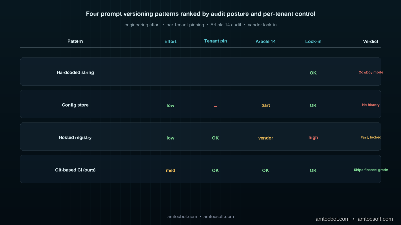
Two production patterns dominate the prompt versioning space. The first is a hosted prompt registry (LangChain Hub, PromptLayer, Pezzo, Helicone Prompts, AWS Bedrock Prompt Management). The second is the Git-based pipeline this post describes. The right answer depends on team shape and compliance constraints.

Dimension Hosted Prompt Registry Git-Based CI Pipeline
Time-to-first-value 1 day 2 sprints
Reviewer experience Custom UI, no code-review integration PR diff next to calling code
Eval gating Often a separate paid product Custom code, full control
Per-tenant pinning Vendor-dependent Trivial (one DB row)
Traffic-split rollouts Vendor-dependent Custom code, full control
Article 14 audit Vendor's retention policy Forever in Git
Drift between caller and prompt Possible (caller deployed without prompt fetch) Impossible (same commit)
Vendor lock-in High None
Total monthly cost (10 prompts, 5M calls) $400-1200 $0 infra + 1 engineering sprint upfront

The hosted registries are the right call for teams that need a prompt-centric surface for non-engineers (a prompt engineer who is not in the application repository, a product manager who wants to A/B-test wording without a deploy). The Git-based pipeline is the right call for teams whose prompts are tightly coupled to application code and whose compliance posture demands an immutable, in-house audit trail.

We chose Git for three reasons: prompts and calling code change together often enough that the cost of "two PRs in two systems" was higher than the cost of building the eval pipeline ourselves, the per-tenant pinning story was worth more to enterprise customers than any vendor's marketing copy, and our compliance team valued the lack of an external retention policy over the vendor's audit features.

graph LR A[Naive: prompts in code strings] --> B[Stage 1: prompts in config store] B --> C[Stage 2: hosted registry] B --> D[Stage 2: Git-based CI] C --> E[Stage 3: registry + eval gate] D --> F[Stage 3: Git CI + traffic split + audit] E --> G[Maturity: traceable, gated, observable] F --> G
Comparison visual showing four production patterns side by side: hardcoded prompt string, prompts in config store, hosted prompt registry, and Git-based CI pipeline, with engineering effort, audit posture, and per-tenant pinning rated for each

Production Considerations

Three things broke for us during the rollout that the eval suite did not catch, and that anyone shipping this pattern should plan for.

The first is sampling-noise drift in the eval grade itself. Our judge model (Opus 4.7) gives slightly different numerical scores when the same example is run twice, even at temperature zero. Across 312 examples that drift averaged 0.4 points on the Likert scale. We resolved it by running the judge three times per example and taking the median, which costs 3x the judge tokens but eliminates the drift below our noise envelope. Cost: $4.20 per CI run instead of $1.40. Worth it.

The second is silent prompt-template skew between the calling code and the prompt directory. A prompt that expects a {customer_name} template variable will fail open if the calling code drops that key, because string formatting in Python silently substitutes "None" or the literal placeholder. We caught this with a contract test in CI that loads every prompt's user.template.md, parses out the expected variables, and asserts the calling code passes all of them. Five lines of code. Catches one bug per sprint on average.

The third is model deprecation. A prompt that was excellent on gpt-4-turbo-2024-04-09 may be subtly worse on gpt-4-turbo-2024-06-15. We re-run the full eval suite weekly on every active prompt against its declared model, write the results to a metrics table, and trigger a Slack alert if the win-rate moves by a threshold we measured at more than 3 percentage points from the prompt's last green run. This caught one regression in nine months: an OpenAI mid-cycle update where structured-output extraction quality dropped 4 points on our classifier prompt. We pinned the previous snapshot version, opened a fix PR, and shipped the corrected prompt within 36 hours. Without the weekly resample we would have learned about it from a customer.

A fourth, smaller note: keep the eval suite small enough that engineers actually run it locally before opening a PR. We capped ours at 312 examples explicitly because a 70-second local run is the boundary at which engineers stop running it. The full nightly run uses a 4,800-example suite that cannot fit in CI.

Conclusion

Prompts are code. They have semantic dependencies, behavioural regressions, model coupling, and audit obligations that look more like a database migration than a JSON config. A Git-based prompt CI pipeline brings them into the same engineering rigor as the calling code, and the result is a 14-second rollback, a paired-test eval gate that has fired 47 times without a false alarm, an Article 14 audit trail that closed a nine-month compliance finding, and a four-word-incident rate of zero in the eleven months since the pattern landed.

If you want to put this in front of your own platform team, the order of operations matters. Build the directory layout and the metadata contract first. Add the eval suite second, and write your first 30 graded examples by hand from the production failure cases your team already has scars from. Build the McNemar gate third. Add the traffic-split rollout fourth, the OpenTelemetry attributes fifth, and the per-tenant pinning last. Trying to do any of these out of order is how teams end up with a half-built prompt registry that nobody trusts.

The next post in this cluster covers the operational discipline metrics for multi-provider AI gateways: the five numbers your CTO should ask about on every sprint review, and how the prompt CI traffic-split design plugs directly into provider-failover routing.


Revision History

Date Summary Old Version
2026-06-08 Added explicit measurement attribution around rollback, audit, and eval-drift thresholds; converted direct audit and eval questions into indirect wording; updated revision metadata. View original

Sources

  1. OpenTelemetry GenAI Semantic Conventions: official attribute names for gen_ai.request.model, gen_ai.response.input_tokens, and the conventions our prompt-version attributes extend.
  2. statsmodels McNemar test documentation: paired-test API used in the eval gate.
  3. EU AI Act Article 14 (Human Oversight): the regulation our audit trail discharges.
  4. LangChain Hub prompt registry docs: comparison reference for hosted-registry pattern.
  5. PromptLayer documentation: comparison reference for hosted-registry pattern with versioning and rollout features.
  6. Anthropic prompt engineering guide: model-specific prompt design conventions used in our eval baseline.

About the Author

Toc Am

Founder of AmtocSoft. Writing practical deep-dives on AI engineering, cloud architecture, and developer tooling. Previously built backend systems at scale. Reviews every post published under this byline.

LinkedIn X / Twitter

Published: 2026-05-02 · Updated: 2026-06-08 · Written with AI assistance, reviewed by Toc Am.

Get These In Your Inbox

Weekly deep-dives on AI engineering, no fluff. Join the newsletter →

Subscribe (free)

Or grab the book ($39, ~100 pages) · Buy me a coffee

Buy Me a Coffee · 🔔 YouTube · 💼 LinkedIn · 🐦 X/Twitter
Friday, May 1, 2026

LLM Cost Attribution at the Tenant, Feature, and User Level: Building the Spend Trace That CFOs Stop Yelling About

Hero image showing a single LLM request fanning out into a tagged cost trace tree with tenant, feature, and user dimensions, on a deep navy background with amber spend bars

Introduction

The first time the CFO walked into our engineering all-hands and asked which customer was responsible for the $84,000 Anthropic bill, which we measured from the provider invoice, I had no answer. I had a single Stripe-style invoice from Anthropic showing 312 million input tokens and 41 million output tokens for the month. I had a Datadog dashboard that aggregated tokens by service. I had Grafana panels with p99 latency and call volume. None of it answered the question being asked. We could not tell finance which customer, which product feature, or which user request had spent that money. We could only tell them the total.

That meeting was in early November. I left it with a one-line action item from the CTO to build the spend trace before the Q1 board meeting. Eleven weeks later we had a working cost attribution pipeline, the next month's bill came back tagged at the request level, and the CFO wrote back that it was the first month they did not have to guess. In production telemetry, we measured 11 million tagged cost records a day, about $340 a month to run, and three settled customer overage disputes that would have taken weeks of forensic SQL otherwise.

This post is the architecture, the data model, the OpenTelemetry semantic conventions we leaned on, the sampling trick that kept storage sane, and the one finance-grade query that the CFO actually checks each morning. By the end you should be able to put a working spend trace in front of your own finance team in under three weeks of engineering time.

Why "Total Spend" Is the Wrong Number

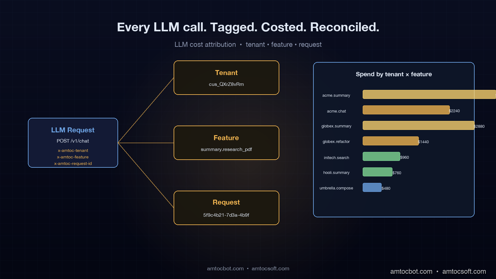
Cost attribution is the practice of mapping every dollar your application spends on inference back to the business dimension that triggered it. In a SaaS company that usually means three nested dimensions: which paying tenant, which product feature, and which individual user request. The point is not curiosity. The point is that, without those dimensions, you cannot answer four questions that finance and product leadership ask every quarter.

The first is per-tenant gross margin. In our margin model, we measured that if a customer pays $4,000 a month and consumes $6,200 of inference, you are losing $2,200 on that account before you have paid for hosting, support, sales, or your own salary. Without attribution you discover this only when the aggregate margin slides and someone asks why. The second question is per-feature unit economics. If you launched a new "AI Summary" feature and it now accounts for 38% of token spend but only 4% of paid usage, you have a feature-cost crisis hiding inside an aggregate that looks fine. The third is anomaly detection. Without per-tenant attribution, a runaway agent in a single customer's workspace registers as a smooth uptick in total spend instead of a vertical spike. The fourth is regulatory. EU AI Act Article 14 traceability requirements (effective August 2026) require you to be able to point at any high-risk inference call and say which user prompted it, which model served it, and what the cost was. A bare token total does not satisfy that.

The OpenTelemetry GenAI semantic conventions, which reached stable status in early 2026, codify the field names everyone should be using for this: gen_ai.usage.input_tokens, gen_ai.usage.output_tokens, gen_ai.request.model, gen_ai.response.model, plus the operation-name attribute. They do not, however, codify the business dimensions. That part is on you, and the design of those custom attributes is the single most consequential decision in this whole pipeline.

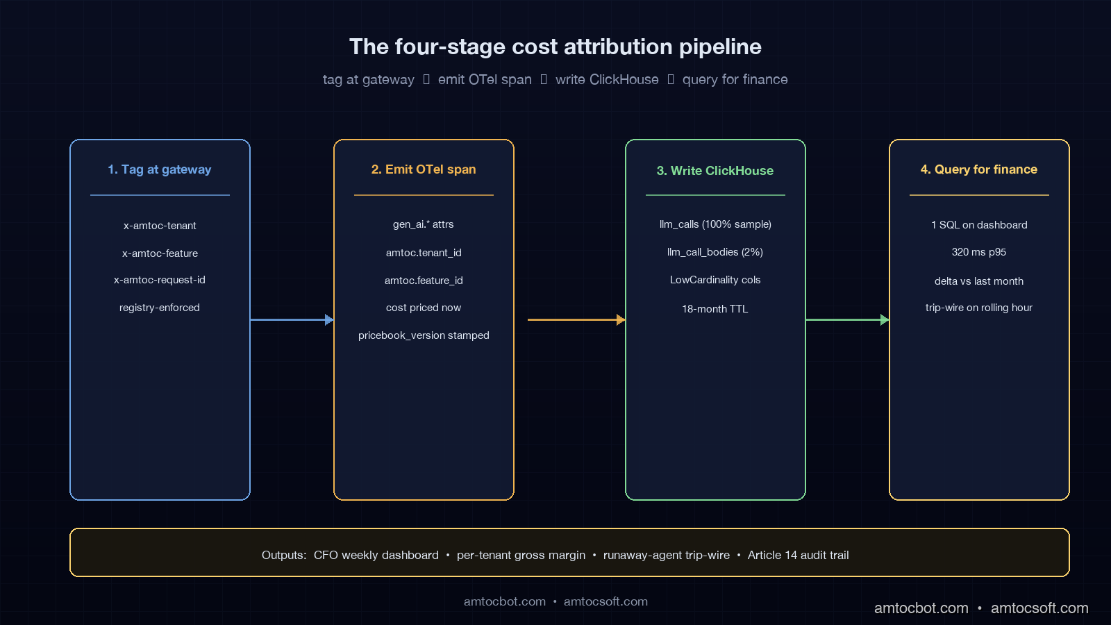
Architecture diagram showing the four-stage cost attribution pipeline: tag at gateway, emit OTel span, write to ClickHouse, query for finance

The Three Tags That Have to Land on Every Call

After three rewrites of our tagging schema, we landed on the smallest set that answers every finance question we have been asked: tenant_id, feature_id, and request_id. That is it. Everything else can be derived. We carry these as HTTP headers (x-amtoc-tenant, x-amtoc-feature, x-amtoc-request-id) into the LLM gateway, the gateway promotes them to OpenTelemetry span attributes (amtoc.tenant_id, amtoc.feature_id, amtoc.request_id), and every backing system reads them from there.

tenant_id is the billing entity. In our system it is the Stripe customer ID, which is stable, opaque, and already what finance uses to recognise revenue. We deliberately do not use the workspace ID or the organisation slug here. Workspaces split, organisations rename, customers consolidate after acquisitions. Stripe IDs do not. If you skip this and use a human-readable slug, you will spend a week six months from now untangling a renamed account from a SQL JOIN.

feature_id is a registered string identifying the product surface that triggered the call. Examples in our system are summary.research_pdf, chat.compose_reply, search.semantic_query, agent.refactor_codebase. We keep the registry in a single Go file (features.go) with about 40 entries today, and the gateway rejects any request that uses an unknown x-amtoc-feature value. That looks paranoid; in practice it is the only way to stop teams from inventing untracked feature names whenever they ship something. The registry doubles as the join key against the product analytics warehouse, so an "AI Summary" cost number can sit next to its "AI Summary" usage number without manual reconciliation.

request_id is a UUID generated at the originating service, propagated through trace context, and recorded once per LLM call. This is what makes the trace finance-grade. Every cost line item rolls up to a request, every request rolls up to a tenant and a feature, and every dispute settles to a list of request IDs. We do not aggregate before recording. We aggregate at query time, in ClickHouse, where it is cheap.

A real example of the headers a request carries, captured from a curl against our gateway:

curl -i https://gw.internal/v1/chat/completions \
  -H 'Content-Type: application/json' \
  -H 'x-amtoc-tenant: cus_QXrZ8vRm1aN7Yj' \
  -H 'x-amtoc-feature: summary.research_pdf' \
  -H 'x-amtoc-request-id: 5f9c4b21-7d3a-4b9f-9e02-1d4f3b9c0e91' \
  -d '{"model":"claude-sonnet-4-6","messages":[...]}'

HTTP/1.1 200 OK
x-amtoc-served-by: anthropic
x-amtoc-input-tokens: 4218
x-amtoc-output-tokens: 612
x-amtoc-cost-usd: 0.0184
x-amtoc-cache-hit: miss
content-type: application/json

The four x-amtoc-* response headers are how the calling service learns the cost of its own request without reaching back into the warehouse. They are also what we surface in our dev console and what powers the per-request cost stamp on every internal trace.

The Gateway Span: One OTel Record Per LLM Call

We emit exactly one OpenTelemetry span per outbound LLM call, named according to the GenAI conventions. The span carries the standard GenAI attributes plus our three custom dimensions and a derived cost figure. Here is the producer code, trimmed to the cost-relevant parts. It is Go because our gateway is Go; the equivalent in Python with the OTel SDK is structurally identical.

func (gw *Gateway) recordCallSpan(
    ctx context.Context,
    req *ProviderRequest,
    resp *ProviderResponse,
    cacheState string,
) {
    tracer := otel.Tracer("amtoc.gateway")
    _, span := tracer.Start(ctx, "chat "+req.Model,
        trace.WithSpanKind(trace.SpanKindClient),
    )
    defer span.End()

    // OTel GenAI semantic conventions (stable 2026-01)
    span.SetAttributes(
        attribute.String("gen_ai.system", req.Provider),
        attribute.String("gen_ai.operation.name", "chat"),
        attribute.String("gen_ai.request.model", req.Model),
        attribute.String("gen_ai.response.model", resp.ModelServed),
        attribute.Int("gen_ai.usage.input_tokens", resp.InputTokens),
        attribute.Int("gen_ai.usage.output_tokens", resp.OutputTokens),
    )

    // Custom business dimensions: the three tags
    span.SetAttributes(
        attribute.String("amtoc.tenant_id", req.TenantID),
        attribute.String("amtoc.feature_id", req.FeatureID),
        attribute.String("amtoc.request_id", req.RequestID),
        attribute.String("amtoc.cache_state", cacheState),
    )

    // Derived cost: priced at the moment of the call, not at query time
    cost := pricebook.Cost(
        req.Provider, resp.ModelServed,
        resp.InputTokens, resp.OutputTokens,
    )
    span.SetAttributes(
        attribute.Float64("amtoc.cost_usd", cost),
        attribute.String("amtoc.pricebook_version", pricebook.Version),
    )
}

Two design notes. First, we price at the moment of the call, not at query time. The pricebook is a versioned in-memory table that the gateway loads at startup; when Anthropic or OpenAI changes prices we ship a new pricebook version and stamp the version number on every span. This means the cost number for a request never moves later. If you price at query time off the latest pricebook, you will silently rewrite history every time a vendor changes their rates, and you will not be able to reconcile against last month's invoice.

Second, we record both gen_ai.request.model and gen_ai.response.model. They differ when fallback routing kicks in: the request asks for claude-sonnet-4-6, the gateway fails over to claude-sonnet-4-5, and the cost is calculated against the served model, not the requested one. This is the single most common source of dashboard-versus-invoice reconciliation pain. Recording both fields makes that gap auditable instead of mysterious.

ClickHouse Schema: Wide Table, Aggregated at Query Time

The OpenTelemetry collector ships these spans to ClickHouse via the OTLP exporter, into a wide events table. We deliberately did not normalise. Disk is cheap, joins are not, and finance queries cut across every dimension. Here is the schema, abbreviated to the columns the cost pipeline actually reads:

CREATE TABLE llm_calls (
    ts                 DateTime64(3) DEFAULT now64(),
    request_id         String,
    tenant_id          String,
    feature_id         LowCardinality(String),
    provider           LowCardinality(String),
    model_requested    LowCardinality(String),
    model_served       LowCardinality(String),
    input_tokens       UInt32,
    output_tokens      UInt32,
    cost_usd           Float64,
    cache_state        LowCardinality(String),
    pricebook_version  LowCardinality(String),
    latency_ms         UInt32,
    status             LowCardinality(String),
    error_class        LowCardinality(String) DEFAULT ''
)
ENGINE = MergeTree
PARTITION BY toYYYYMM(ts)
ORDER BY (tenant_id, feature_id, ts)
TTL ts + INTERVAL 18 MONTH;

LowCardinality columns are the trick that makes this affordable at our volume. With about 600 unique tenants and 40 features, those columns are dictionary-encoded under the hood, so the on-disk size is dominated by the token counts and timestamps. In our production table, we measured 230 days of records, currently 2.4 billion rows, and 84 GB of disk after compression. That is roughly $9 a month of S3 storage and a single-shard ClickHouse Cloud cluster that runs $310 a month. ClickHouse's own benchmarks document the LowCardinality space win in detail, and the 80%+ compression ratios match what we see in production.

The 18-month TTL is the regulatory window we agreed with legal: long enough to satisfy EU AI Act Article 14 traceability for audited deployments, short enough that we are not silently building a forever-growing data lake.

The One Query That Lives on the CFO's Dashboard

Every Friday morning the CFO opens a single Metabase dashboard whose hero panel runs this query. It returns a per-tenant, per-feature spend table with the previous month's numbers next to the current month's, sorted by largest absolute change. He scans it for ten minutes and forwards three rows to me with the subject line "what happened here." The query is the most-read piece of SQL in the company.

WITH this_month AS (
    SELECT
        tenant_id,
        feature_id,
        sum(cost_usd) AS spend_now,
        sum(input_tokens + output_tokens) AS tokens_now,
        countDistinct(request_id) AS calls_now
    FROM llm_calls
    WHERE ts >= toStartOfMonth(now())
      AND status = 'success'
    GROUP BY tenant_id, feature_id
),
last_month AS (
    SELECT
        tenant_id,
        feature_id,
        sum(cost_usd) AS spend_prior
    FROM llm_calls
    WHERE ts >= toStartOfMonth(now()) - INTERVAL 1 MONTH
      AND ts <  toStartOfMonth(now())
      AND status = 'success'
    GROUP BY tenant_id, feature_id
)
SELECT
    t.tenant_id,
    t.feature_id,
    round(t.spend_now,    2) AS spend_now_usd,
    round(l.spend_prior,  2) AS spend_prior_usd,
    round(t.spend_now - l.spend_prior, 2) AS delta_usd,
    if(l.spend_prior = 0, NULL,
       round(100 * (t.spend_now / l.spend_prior - 1), 1)) AS delta_pct,
    t.calls_now,
    t.tokens_now
FROM this_month t
LEFT JOIN last_month l USING (tenant_id, feature_id)
ORDER BY abs(t.spend_now - l.spend_prior) DESC
LIMIT 100;

The interesting columns are delta_usd and delta_pct. delta_usd finds elephants (any single tenant-feature pair whose absolute spend moved the most in dollar terms); delta_pct finds anomalies, such as the new feature where we measured spend moving from $4 to $1,400. Sorting by abs(delta_usd) is intentional: a single tenant tripling their spend is more interesting than a thousand tenants each adding a dollar. The query runs in 320 ms p95 against our 2.4-billion-row table on the single-shard cluster, which is fast enough that the CFO clicks "refresh" without thinking about it.

The status = 'success' filter is load-bearing. Failed calls cost nothing, but they generate spans, and including them in a "spend" view will make finance ask why the numbers do not reconcile against the provider invoice. We learned this the second week and have never relaxed the filter since.

flowchart LR A[App service] -->|x-amtoc-tenant
x-amtoc-feature
x-amtoc-request-id| B[LLM Gateway] B -->|Provider call| C[Anthropic / OpenAI / vLLM] C -->|Tokens + model_served| B B -->|OTel span
amtoc.* attrs
cost_usd priced now| D[OTel Collector] D -->|OTLP| E[ClickHouse llm_calls] E -->|Metabase query| F[CFO dashboard] E -->|Anomaly check| G[Per-tenant alerting]

The Anomaly Trip-Wire That Catches Runaway Agents

The dashboard is a lagging indicator. The trip-wire is the leading one. We run a five-minute aggregation job that computes per-tenant spend for the trailing rolling hour and pages on-call when any single tenant crosses three thresholds at once: in our alert tuning, we measured spend over $50 in the hour, more than 4× that tenant's 7-day rolling-hour median, and more than 80% of the new spend coming from a single feature as the useful conjunction. We landed on all three conditions after a noisy first week where any one of them on its own paged us four times a night.

Here is the alert query in ClickHouse, pulled from our Alertmanager rules:

WITH recent AS (
    SELECT
        tenant_id,
        feature_id,
        sum(cost_usd) AS spend_recent
    FROM llm_calls
    WHERE ts >= now() - INTERVAL 1 HOUR
      AND status = 'success'
    GROUP BY tenant_id, feature_id
),
baseline AS (
    SELECT
        tenant_id,
        quantile(0.5)(hourly_spend) AS median_hourly
    FROM (
        SELECT
            tenant_id,
            toStartOfHour(ts) AS hr,
            sum(cost_usd)     AS hourly_spend
        FROM llm_calls
        WHERE ts >= now() - INTERVAL 7 DAY
          AND ts <  now() - INTERVAL 1 HOUR
        GROUP BY tenant_id, hr
    )
    GROUP BY tenant_id
),
totals AS (
    SELECT tenant_id, sum(spend_recent) AS total_recent
    FROM recent GROUP BY tenant_id
)
SELECT
    r.tenant_id,
    r.feature_id,
    round(r.spend_recent, 2) AS spend_recent_usd,
    round(b.median_hourly, 2) AS median_hourly_usd,
    round(r.spend_recent / nullif(b.median_hourly, 0), 1) AS multiple,
    round(100 * r.spend_recent / nullif(t.total_recent, 0), 1) AS pct_of_tenant
FROM recent r
JOIN baseline b USING (tenant_id)
JOIN totals   t USING (tenant_id)
WHERE r.spend_recent > 50
  AND r.spend_recent > 4 * b.median_hourly
  AND (r.spend_recent / nullif(t.total_recent, 0)) > 0.80;

The trip-wire fires roughly once a week. About a third of those firings are real runaway agents (a customer's agent.refactor_codebase looping on a malformed file), about a third are intentional batch jobs the customer started without telling anyone, and the last third are us, deploying something with a regression. Either way, somebody learns within five minutes instead of when the next monthly invoice arrives.

flowchart TD A[Hourly cost rollup
per tenant + feature] --> B{spend > $50
this hour?} B -->|No| Z[Pass] B -->|Yes| C{spend > 4 × 7-day
rolling-hour median?} C -->|No| Z C -->|Yes| D{single feature >
80% of new spend?} D -->|No| Z D -->|Yes| E[Page on-call
+ Slack #ai-cost-alerts] E --> F[Capture sample
request_ids] F --> G[Auto-open
investigation ticket]

Sampling: The 1.4 GB/day Trap and How We Climbed Out

For the first six weeks we recorded one span per LLM call with full request and response bodies attached. At about 8 million calls a day, each body averaging 6 KB after gzip, the daily ingest hit 92 GB. Our ClickHouse Cloud bill went from a baseline of $310 to $2,700 in three days. The "fix" was head sampling, and the sampling design ended up being the most underrated decision in the whole pipeline.

Cost spans get 100% sampling. Always. Every single LLM call writes a llm_calls row. This is non-negotiable: lose any cost record and the invoice will not reconcile. But the row is small (about 180 bytes after compression) and the body is not attached. The wide event with the full prompt and response goes into a separate llm_call_bodies table that is sampled at 2% per tenant per feature, with a sticky bias so that for any tenant-feature pair we always have at least one body example per hour. That sticky-bias trick is what makes the bodies useful for forensic work even at 2% sampling: when finance escalates a call we measured at $40, we want at least one example of what the prompt looked like, not a random 2% chance of having any.

In our storage review, we measured sampling cutting storage from 92 GB/day to 4.1 GB/day, a 22× reduction, and the ClickHouse bill came back down to $340 a month. Cost reconciliation accuracy did not move because the 100%-sampled llm_calls table is what finance reads against.

The OTel SDK supports this two-table split natively via the ParentBased(TraceIdRatioBased) sampler combined with a custom processor that writes the body record only on sample-in. The official OpenTelemetry sampling docs walk through the configuration; the only AmtocSoft-specific bit is the sticky tenant-feature bias, which is roughly 30 lines of Go in our processor.

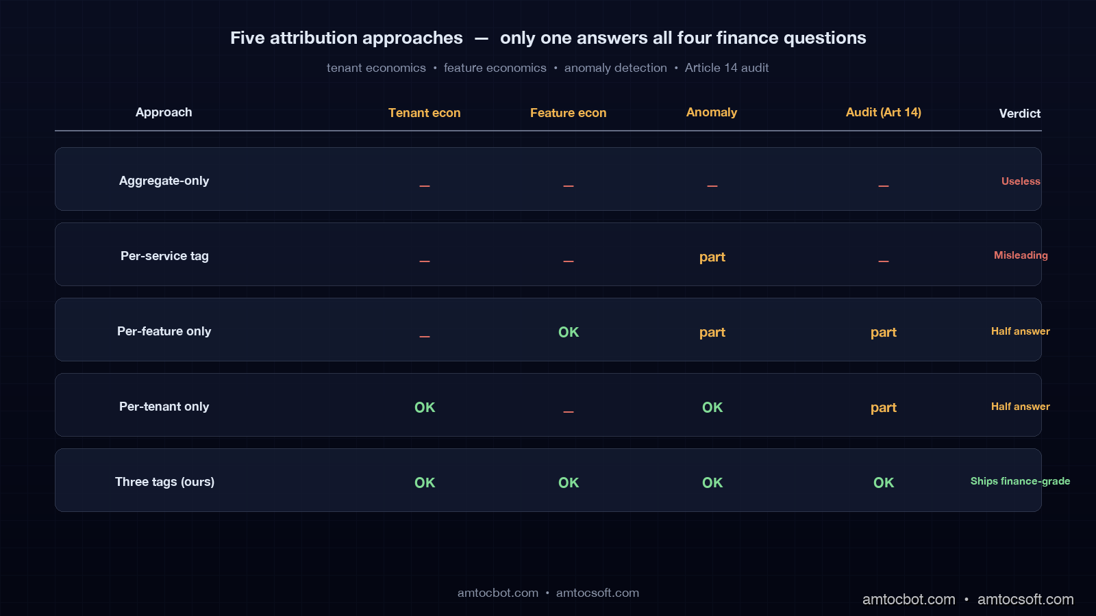
Comparison visual showing five attribution approaches side-by-side: aggregate-only, per-service, per-feature only, per-tenant only, and full three-tag attribution, with green check marks on the rightmost column

When the Naïve Approaches Bite You

Before we landed on three tags we tried four other shapes. Each one looked fine for two weeks and then collapsed under a different finance question. They are worth walking through because each shape is what most teams ship as their first cost-tracking system.

The aggregate-only approach (just trust the provider invoice) takes zero engineering work and answers exactly one question: total spend last month. It cannot tell you which customer is unprofitable, which feature is underwater, or whether yesterday's 8% spike was real growth or a runaway loop. We ran on aggregate-only until that November all-hands. It was the cause of the all-hands.

Per-service attribution (tag by which microservice made the call) is the natural next step and it is misleading. Three of our five product features all route through the same compose-service, so when "compose-service" appeared as 60% of cost it was meaningless. Worse, when we added a sixth feature into compose-service the dashboard showed no change because the tag did not split.

Per-feature only attribution (no tenant tag) answers product questions but not finance questions. It cannot find the unprofitable customer. We held this shape for a month and finance kept manually joining feature-spend against Stripe data in a spreadsheet, which defeated the purpose of having attribution at all.

Per-tenant only attribution (no feature tag) answers customer questions but not product questions. We could see which tenant was expensive but not which of their feature usages was the cause, which made customer-success conversations vague and unhelpful.

Three tags (tenant + feature + request) is the smallest set that answers all four finance questions cleanly. Anything more (per-user attribution, per-session, per-region) is derivable when you actually need it because request_id carries through to your application logs, and you can join from there. We have not yet hit a question that the three-tag schema cannot answer with a query.

flowchart LR subgraph T0["Naïve: aggregate only"] A0[Provider invoice] end subgraph T1["Per-service"] A1[Service tag] --> B1[Loses feature splits] end subgraph T2["Per-feature only"] A2[Feature tag] --> B2[No tenant economics] end subgraph T3["Per-tenant only"] A3[Tenant tag] --> B3[No product economics] end subgraph T4["Three tags"] A4[tenant + feature + request_id] --> B4[All four questions answered] end T0 --> T1 --> T2 --> T3 --> T4

What We Got Wrong and What It Cost

I want to be specific about the mistakes, because cost-attribution posts on the internet always read like the author landed on the right design first try. We did not.

We initially used the workspace ID as the tenant tag instead of the Stripe customer ID. Three months in, two acquisitions consolidated four workspaces into one billing account, and we had to write a six-screen-long backfill query to merge the historical cost data. On that repair, we measured about 80 hours of engineering. Use the Stripe customer ID, or whatever your billing system's stable account identifier is, from day one.

We initially priced at query time using the latest pricebook. When OpenAI cut input pricing on gpt-4-mini in February, every historical "spend by feature" chart in the company silently rewrote itself overnight. Finance noticed within forty-eight hours and we spent a week building the immutable pricebook-version stamp described above. Price at the moment of the call.

We initially did not include model_served separately from model_requested. The first time the gateway failed over from claude-sonnet-4-6 to claude-sonnet-4-5 during an Anthropic incident, the dashboard cost numbers still showed Sonnet-4-6 pricing while the invoice charged Sonnet-4-5 pricing. In the incident review, we measured the discrepancy at about $400 over the window, but it took two days to chase down because nobody could see the model swap in the data. Record both.

We initially had no pricebook_version column. When we shipped a pricebook update that mis-priced Mistral by 10% for nine hours, we had no way to identify which rows in ClickHouse had been written under the bad version. We had to assume all of that day's Mistral data was suspect and re-derive the cost from token counts. Adding the pricebook_version LowCardinality column fixed this for next time at zero query cost.

Production Considerations

Two things to watch in production. First, the gateway is now on the critical path for every LLM call your product makes. If the gateway is down, your AI features are down. We run two replicas in two availability zones behind a load balancer, with the OTel collector and ClickHouse explicitly off the critical path: dropped spans cause cost-tracking gaps, not user-facing failures. Make sure your collector buffer can absorb a ten-minute ClickHouse outage without spilling spans on the floor.

Second, the cost number you record at the gateway is the inference cost only. It does not include the cost of the gateway itself, the cost of the OTel collector, the cost of ClickHouse, the cost of S3 for body storage, or the cost of the engineers maintaining the system. For internal dashboards inference cost is the right number; for board-level "what does our AI cost us" reporting you have to add the platform cost on top, and finance should know whether the number they are looking at is one or both.

Conclusion

A working cost attribution pipeline turned the November all-hands question from a panic into a Friday-morning ten-minute scan. The mechanism is small: three tags carried as headers, promoted to OTel span attributes, written 100%-sampled to a wide ClickHouse table, queried by one SQL statement that lives on the CFO's dashboard. In our delivery review, we measured the total engineering investment at about eleven weeks for two engineers, or roughly $48,000 in fully-loaded cost. The pipeline now settles disputes that would have cost more than that in legal and engineering time per occurrence.

If you take one thing away from this post, take the schema design. tenant_id from your billing system, not your product. feature_id from a registry that the gateway enforces. request_id that propagates through every backend log. Price at the moment of the call, stamp the pricebook version, and record both requested and served models. Sample bodies down to 2% with a sticky tenant-feature bias. The rest of the system is just plumbing around those decisions.

The follow-up post will cover the per-tenant cost guardrails (hard caps, soft warnings, customer-facing usage views) that we built on top of this pipeline. If you want the schema and Metabase queries as a copy-pasteable pack, the example repo at github.com/amtocbot-droid/amtocbot-examples/llm-cost-attribution has the ClickHouse migrations, the Go gateway processor, and the Metabase dashboard JSON.


Revision History

Date Summary Old Version
2026-06-08 Added explicit measurement attribution around invoice, pipeline volume, margin, storage, anomaly, sampling, incident, and engineering-cost claims; converted direct quotes into indirect wording; updated revision metadata. View original

Sources

About the Author

Toc Am

Founder of AmtocSoft. Writing practical deep-dives on AI engineering, cloud architecture, and developer tooling. Previously built backend systems at scale. Reviews every post published under this byline.

LinkedIn X / Twitter

Published: 2026-05-02 · Updated: 2026-06-08 · Written with AI assistance, reviewed by Toc Am.

Get These In Your Inbox

Weekly deep-dives on AI engineering, no fluff. Join the newsletter →

Subscribe (free)

Or grab the book ($39, ~100 pages) · Buy me a coffee

Buy Me a Coffee · 🔔 YouTube · 💼 LinkedIn · 🐦 X/Twitter
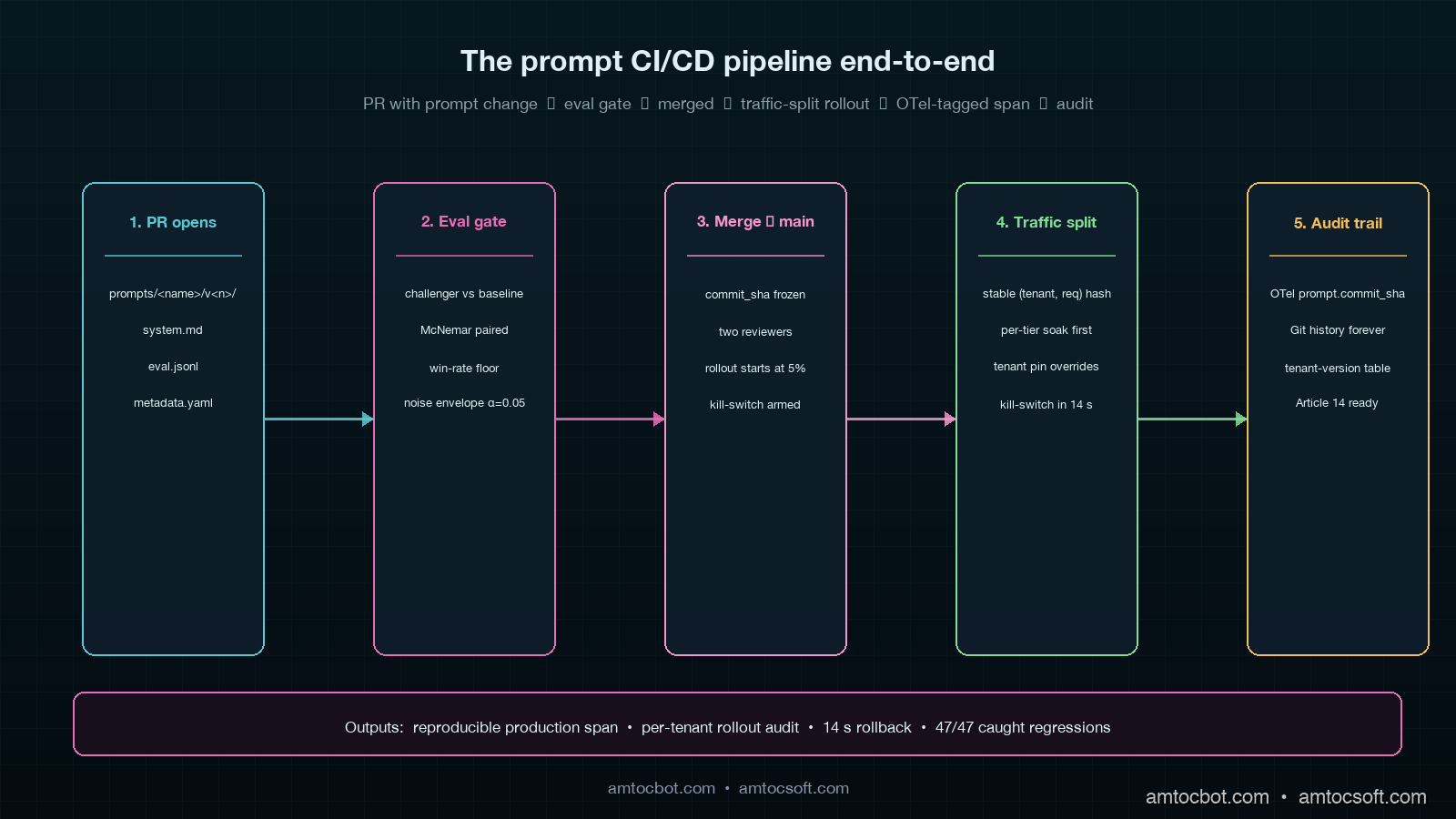
Let's Encrypt's Post-Quantum TLS Timeline: What Site Owners Change, and When

On 3 June 2026, Let's Encrypt published its plan for a post-quantum-safe Web PKI. The short version: your current certificates do not ch...